I use this all the time, and the setup is dead simple. Follow the code below to load the RMySQL package, connect to a database (here the UCSC genome browser's public MySQL instance), set up a function to make querying easier, and query the database to return results as a data frame.
Thursday, December 15, 2011
Galaxy Project Group on CiteULike and Mendeley

While not a CUL user, I'm a big fan of Mendeley for managing references, PDFs, and creating bibliographies (and so are many of you). I'm happy to hear that the Galaxy folks also set up a Galaxy Mendeley Group, also open to the public for anyone to join. If you join the Galaxy public Mendeley group, all of the groups references will show up in your Mendeley library (and these won't count against your personal quota).

Just one important thing to note: The Mendeley group is a mirror of the CiteULike group, so if you want to add more publications to the Galaxy Group, add them on CiteULike, not Mendeley (it doesn't work the other way around - papers added to Mendeley won't make it to the CUL group).
Galaxy Project Group on CiteULike and Mendeley
Thursday, December 8, 2011
RNA-Seq & ChiP-Seq Data Analysis Course at EBI
I just got this announcement from EMBL-EBI about an RNA-seq/ChIP-seq analysis hands-on course. Find the full details, schedule, and speaker list here.
Title: Advanced RNA-Seq and Chip-Seq Data Analysis Course
Date: May 1-4 2012
Venue: EMBL-EBI, Hinxton, Nr Cambridge, CB10 1SD, UK
Registration Closing Date: March 6 2012 (12:00 midday GMT)
This course is aimed at advanced PhD students and post-doctoral researchers who are applying or planning to apply high throughput sequencing technologies and bioinformatics methods in their research. The aim of this course is to familiarize the participants with advanced data analysis methodologies and provide hands-on training on the latest analytical approaches.
Lectures will give insight into how biological knowledge can be generated from RNA-seq and ChIP-seq experiments and illustrate different ways of analyzing such data Practicals will consist of computer exercises that will enable the participants to apply statistical methods to the analysis of RNA-seq and ChIP-seq data under the guidance of the lecturers and teaching assistants. Familiarity with the technology and biological use cases of high throughput sequencing is required, as is some experience with R/Bioconductor.
The course covers data analysis of RNA-Seq and ChIP-Seq experiments.
Topics will include: alignment, data handling and visualisation, region identification, differential expression, data quality assessment and statistical analysis, using R/Bioconductor.
Tuesday, December 6, 2011
An example RNA-Seq Quality Control and Analysis Workflow
I found the slides below on the education page from Bioinformatics & Research Computing at the Whitehead Institute. The first set (PDF) gives an overview of the methods and software available for quality assessment of microarray and RNA-seq experiments using the FastX toolkit and FastQC.
The second set (PDF) gives an example RNA-seq workflow using TopHat, SAMtools, Python/HTseq, and R/DEseq.
If you're doing any RNA-seq work these are both really nice resources to help you get a command-line based analysis workflow up and running (if you're not using Galaxy for RNA-seq).
The second set (PDF) gives an example RNA-seq workflow using TopHat, SAMtools, Python/HTseq, and R/DEseq.
If you're doing any RNA-seq work these are both really nice resources to help you get a command-line based analysis workflow up and running (if you're not using Galaxy for RNA-seq).
Monday, December 5, 2011
Webinar: Applications of Next-Generation Sequencing in Clinical Care
I just got an email from Illumina about a webinar that looks interesting this Wednesday at 9am PST (noon EST) on clinical applications of next-gen sequencing.
Date: Wednesday, December 7, 2011
Time: 9:00 AM (PST)
Speaker: Rick Dewey, MD, Stanford Center for Inherited Cardiovascular Disease
Next-generation sequencing (NGS) presents both challenges and opportunities for clinical care. Dr. Dewey will share examples from his experience at Stanford, successful and otherwise, in which NGS has been applied to cases of familial cardiomyopathy, and other inherited conditions. Bring your questions for a Q&A session. In this webinar, Dr. Dewey will discuss approaches to: Data storage and management; Error identification and reduction; Disease risk encoded in the reference sequence; and Variant validation.
The webinar will be recorded and available to you afterwards if you register.
Registration - Applications of Next-Generation Sequencing in Clinical Care
Friday, November 18, 2011
BioMart Gene ID Converter
BioMart recently got a facelift. I'm not sure if this was always available in the old BioMart, but there's now a link to a gene ID converter that worked pretty well for me for converting S. cerevisiae gene IDs to standard gene names. It looks like the tool will convert nearly any ID you could imagine. Looks like it will also map Affy probe IDs to gene, transcript, or protein IDs and names.

BioMart Gene ID Converter
BioMart Gene ID Converter
Thursday, November 17, 2011
GEO2R: Web App to Analyze Gene Expression in GEO Datasets Using R
Gene Expression Omnibus is NCBI's repository for publicly available gene expression data with thousands of datasets having over 600,000 samples with array or sequencing data. You can download data from GEO using FTP, or download and load the data directly into R using the GEOquery bioconductor package written (and well documented) by Sean Davis, and analyze the data using the limma package.
GEO2R is a very nice web-based tool to do this graphically and automatically. Enter the GEO series number in the search box (or use this one for an example). Start by creating groups (e.g. control vs treatment, early vs late time points in a time course, etc), then select samples to add to that group.

Scroll down to the bottom and click Top 250 to run an analysis in limma (the users guide documents this well). GEO2R will automatically fetch the data, group your samples, create your design matrix for your differential expression analysis, run the analysis, and annotate the results. A big complaint with point-and-click GUI and web based applications is the lack of reproducibility. GEO2R obviates this problem by giving you all the R code it generated to run the analysis. Click the R script tab to see the R code it generated, and save it for later.
The options tab allows you to adjust the multiple testing correction method, and the value distribution tab lets you take a look at the distribution gene expression values among the samples that you assigned to your groups.

There's no built-in quality assessment tools in GEO2R, but you can always take the R code it generated and do your own QA/QC. It's also important to verify what values it's pulling from each array into the data matrix. In this example, epithelial cells at various time points were compared to a reference cell line, and the log base 2 fold change was calculated. This was used in the data matrix rather than the actual expression values.
GEO2R is a very nice tool to quickly run an analysis on data in GEO. Now, if we could only see something similar for the European repository, ArrayExpress.
GEO2R: Web App to Analyze Gene Expression in GEO Datasets Using R
GEO2R is a very nice web-based tool to do this graphically and automatically. Enter the GEO series number in the search box (or use this one for an example). Start by creating groups (e.g. control vs treatment, early vs late time points in a time course, etc), then select samples to add to that group.
Scroll down to the bottom and click Top 250 to run an analysis in limma (the users guide documents this well). GEO2R will automatically fetch the data, group your samples, create your design matrix for your differential expression analysis, run the analysis, and annotate the results. A big complaint with point-and-click GUI and web based applications is the lack of reproducibility. GEO2R obviates this problem by giving you all the R code it generated to run the analysis. Click the R script tab to see the R code it generated, and save it for later.
The options tab allows you to adjust the multiple testing correction method, and the value distribution tab lets you take a look at the distribution gene expression values among the samples that you assigned to your groups.
There's no built-in quality assessment tools in GEO2R, but you can always take the R code it generated and do your own QA/QC. It's also important to verify what values it's pulling from each array into the data matrix. In this example, epithelial cells at various time points were compared to a reference cell line, and the log base 2 fold change was calculated. This was used in the data matrix rather than the actual expression values.
GEO2R is a very nice tool to quickly run an analysis on data in GEO. Now, if we could only see something similar for the European repository, ArrayExpress.
GEO2R: Web App to Analyze Gene Expression in GEO Datasets Using R
Tuesday, November 1, 2011
Guide to RNA-seq Analysis in Galaxy
James Taylor came to UVA last week and gave an excellent talk on how Galaxy enables transparent and reproducible research in genomics. I'm gearing up to take on several projects that involve next-generation sequencing, and I'm considering installing my own Galaxy framework on a local cluster or on the cloud.
If you've used Galaxy in the past you're probably aware that it allows you to share data, workflows, and histories with other users. New to me was the pages section, where an entire analysis is packaged on a single pages, and vetting is crowdsourced to other Galaxy users in the form of comments and voting.
I recently found a page published by Galaxy user Jeremy that serves as a guide to RNA-seq analysis using Galaxy. If you've never done RNA-seq before it's a great place to start. The guide has all the data you need to get started on an experiment where you'll use TopHat/Bowtie to align reads to a reference genome, and Cufflinks to assemble transcripts and quantify differential gene expression, alternative splicing, etc. The dataset is small, so all the analyses start and finish quickly, allowing you to finish the tutorial in just a few hours. The author was kind enough to include links to relevant sections of the TopHat and Cufflinks documentation where it's needed in the tutorial. Hit the link below to get started.
Galaxy Pages: RNA-seq Analysis Exercise
Thursday, October 27, 2011
A New Dimension to Principal Components Analysis
In general, the standard practice for correcting for population stratification in genetic studies is to use principal components analysis (PCA) to categorize samples along different ethnic axes. Price et al. published on this in 2006, and since then PCA plots are a common component of many published GWAS studies. One key advantage to using PCA for ethnicity is that each sample is given coordinates in a multidimensional space corresponding to the varying components of their ethnic ancestry. Using either full GWAS data or a set of ancestral informative markers (AIMs), PCA can be easily conducted using available software packages like EIGENSOFT or GCTA. HapMap samples are sometimes included in the PCA analysis to provide a frame of reference for the ethnic groups.
Once computed, each sample will have values that correspond to a position in the new coordinate system that effectively clusters samples together by ethnic similarity. The results of this analysis are usually plotted/visualized to identify ethnic outliers or to simply examine the structure of the data. A common problem however is that it may take more than the first two principal components to identify groups.
To illustrate, I will plot some PCs generated based on 125 AIMs markers for a recent study of ours. I generated these using GCTA software and loaded the top 5 PCs into R using the read.table() function. I loaded the top 5, but for continental ancestry, I've found that the top 3 are usually enough to separate groups. The values look something like this:
new_ruid pc1 pc2 pc3 pc4 pc5
1 11596 4.10996e-03 -0.002883830 0.003100840 -0.00638232 0.00709780
2 5415 3.22958e-03 -0.000299851 -0.005358910 0.00660643 0.00430520
3 11597 -4.35116e-03 0.013282400 0.006398130 0.01721600 -0.02275470
4 5416 4.01592e-03 0.001408180 0.005077310 0.00159497 0.00394816
5 3111 3.04779e-03 -0.002079510 -0.000127967 -0.00420436 0.01257460
6 11598 6.15318e-06 -0.000279919 0.001060880 0.00606267 0.00954331
I loaded this into a dataframe called pca, so I can plot the first two PCs using this command:
plot(pca$pc1, pca$pc2)

We might also want to look at the next two PCs:
plot(pca$pc2, pca$pc3)

Its probably best to look at all of them together:
pairs(pca[2:4])

So this is where my mind plays tricks on me. I can't make much sense out of these plots -- there should be four ethnic groups represented, but its hard to see who goes where. To look at all of these dimensions simultaneously, we need a 3D plot. Now 3D plots (especially 3D scatterplots) aren't highly regarded -- in fact I hear that some poor soul at the University of Washington gets laughed at for showing his 3D plots -- but in this case I found them quite useful.
Using a library called rgl, I generated a 3D scatterplot like so:
plot3d(pca[2:4])

Now, using the mouse I could rotate and play with the cloud of data points, and it became more clear how the ethnic groups sorted out. Just to double check my intuition, I ran a model-based clustering algorithm (mclust) on the data. Different parameters obviously produce different cluster patterns, but I found that using an "ellipsoidal model with equal variances" and a cluster size of 4 identified the groups I thought should be there based on the overlay with the HapMap samples.
fit <- Mclust(pca[2:4], G=4, modelNames = "EEV")
plot3d(pca[2:4], col = fit$classification)

plot(pca[2:3], cex = fit$uncertainty*10)

Tuesday, October 18, 2011
My thoughts on ICHG 2011

On Wednesday, Marylyn Ritchie(@MarylynRitchie) and Nancy Cox organized “Beyond Genome-wide association studies”. Nancy Cox presented some ideas on how to integrate multiple “intermediate” associations for SNPs, such as expression QTLs and newly discovered protein QTLs (More on pQTLs later). This approach which she called a Functional Unit Analysis would group signals together based on the genes they influence. Nicholas Shork presented some nice examples of pros and cons of sequence level annotation algorithms. Trey Idekker gave a very nice talk illustrating some of the properties of epistasis in yeast protein interaction networks. One of the more striking points he made was that epistasis tends to occur between full protein complexes rather than within elements of the complexes themselves. Marylyn Ritchie presented the ideas behind her ATHENA software for machine learning analysis of genetic data, and Manuel Mattesian from Tim Becker’s group presented the methods in their INTERSNP software for doing large-scale interaction analysis. What was most impressive with this session is that there were clear attempts to incorporate underlying biological complexity into data analysis.
On Thursday, I attended the second Statistical Genetics section called “Expanding Genome-wide Association Studies”, organized by Saurabh Ghosh and Daniel Shriner. Having recently attended IGES, I feel pretty “up” on newer analysis techniques, but this session had a few talks that sparked my interest. The first three talks were related to haplotype phasing and the issues surrounding computational accuracy and speed. The basic goal of all these methods is to efficiently estimate genotypes for a common set of loci for all samples of a study using a set of reference haplotypes, usually from the HapMap or 1000 genomes data. Despite these advances, it seems like phasing haplotypes for thousands of samples is still a massive undertaking that requires a high-performance computing cluster. There were several talks about ongoing epidemiological studies, including the Kaiser Permanente UCSF cohort. Neil Risch presented an elegant study design implementing four custom GWAS chips for the four targeted populations. Looks like the data hasn't started to flow from this yet, but when it does we’re sure to learn about lots of interesting ethnic-specific disease effects. My good friend and colleague Dana Crawford presented an in silico GWAS study of hypothyroidism. In her best NPR voice, Dana showed how electronic medical records with GWAS data in the EMERGE network can be re-used to construct entirely new studies nested within the data collected for other specific disease purposes. Her excellent Post-Doc, Logan Dumitrescu presented several gene-environment interactions between Lipid levels and vitamin A and E from Dana’s EAGLE study. Finally Paul O’Reilly presented a cool new way to look at multiple phenotypes by essentially flipping a typical regression equation around, estimating coefficients that relate each phenotype in a study to a single SNP genotype as an outcome. This rather clever approach called MultiPhen is similar to log-linear models I’ve seen used for transmission-based analysis, and allows you to model the “interaction” among phenotypes in much the same way you would look at SNP interactions.
By far the most interesting talks of the meeting (for me) were in the Genomics section on Gene Expression, organized by Tomi Pastinen and Mark Corbett. Chris Mason started the session off with a fantastic demonstration of the power of RNA-seq. Examining transcriptomes of 14 non-human primate species, they validated many of the computational predictions in the AceView gene build, and illustrated that most “exome” sequencing is probably examining less than half of all transcribed sequences. Rupali Patwardhan talked about a system for examining the impact of promoter and enhancer mutations in whole mice, essentially using mutagenesis screens to localize these regions. Ron Hause presented work on the protein QTLs that Nancy Cox alluded to earlier in the conference. Using a high-throughput form of western blots, they systematically examined levels for over 400 proteins in the Yoruba HapMap cell lines. They also illustrate that only about 50% of eQTLs identified in these lines actually alter protein levels. Stephen Montgomery spoke about the impact of rare genetic variants within a transcript on transcript levels. Essentially he showed an epistatic effect on expression, where transcripts with deleterious alleles are less likely to be expressed – an intuitive and fascinating finding, especially for those considering rare-variant analysis. Athma Pai presented a new QTL that influences mRNA decay rates. By measuring multiple time points using RNA-seq, she found individual-level variants that alter decay, which she calls dQTLs. Veronique Adoue looked at cis-eQTLs relative to transcription factor binding sites using ChIP, and Alfonso Buil showed how genetic variants influence gene expression networks (or correlation among gene expression) across tissue types.
I must say despite all the awesome work presented in this session, Michael Snyder stole the show with his talk on the “Snyderome” – his own personal –omics profile collected over 21 months. His whole-genome was sequenced by Complete Genomics, and processed using Rong Chen and Atul Butte’s risk-o-gram to quantify his disease risk. His profile predicted increased risk of T2D, so he began collecting glucose measures and low and behold, he saw a sustained spike in blood glucose levels following a few days following a common cold. His interpretation was that an environmental stress knocked him into a pseudo-diabetic state, and his transcriptome and proteome results corroborated this idea. Granted, this is an N of 1, and there is still lots of work to be done before this type of analysis revolutionizes medicine, but the take home message is salient – multiple -omics are better than one, and everyone’s manifestation of a complex disease is different. This was truly thought-provoking work, and it nicely closed an entire session devoted to understanding the intermediate impact of genetic variants to better understand disease complexity.
This is just my take of a really great meeting -- I'm sure I missed lots of excellent talks. If you saw something good please leave a comment and share!
Saturday, October 8, 2011
Find me at ICHG!
This week, I'm off to Montreal for the International Congress on Human Genetics and I hope to see you there!
If you are attending and are already a part of the Twitterverse, bring a tablet or phone and tweet away about the meeting using the official hashtag, #ICHG2011. If you are new to twitter, go sign up! Using nearly any twitter application, you can search for tweets that contain the #ICHG2011 hashtag and follow the thoughts of your fellow conference goers.
Using Twitter at an academic conference is a fascinating experience! Not only can you get fantastic information about what is being presented at the multitude of sessions, you get lots of opinion on what is going on in the field, and sometimes practically useful tips, like the location of the nearest Starbucks.
If you see me wandering aimlessly around the conference center, please come say hello! Its always great to make new academic friends.
See you there!
Will
Thursday, September 29, 2011
The Utility of Network Analysis
Like most bioinformatics nerds (or anyone with a facebook account), I’m fascinated by networks. Most people immediately think of protein-protein interaction networks, or biological pathways when thinking about networks, but sometimes representing a problem as a network makes solving problems easier.
Recently, some collaborators from the PAGE study had a list of a few hundred SNPs gathered from multiple loci across the genome. For analysis purposes, they were interested in quantifying the number of loci these SNPs represented – in other words, how many distinct signals were represented by their collection of SNPs.
We had linkage disequilibrium data from the HapMap for all pairs of SNPs, and we filtered this using an r-squared cutoff. What we were left with was a mess of SNP pairs that could be tedious to sort through in a spreadsheet. Instead, I represented each pair of SNPs as an edge in a network and loaded the data into Gephi, which provides some wonderful analysis tools. Suppose my LD data is structured like this:
In a spreadsheet application, I sorted and filtered the LD pairings I wanted using either the r-squared or the d-prime columns. I then deleted any rows that didn’t meet my cutoff, renamed the header for SNP1 to “Source” and SNP2 to “Target”, and exported the file as a comma-separated file (.csv). I opened Gephi, clicked the “Data Laboratory” tab, and Import Spreadsheet to load my data.
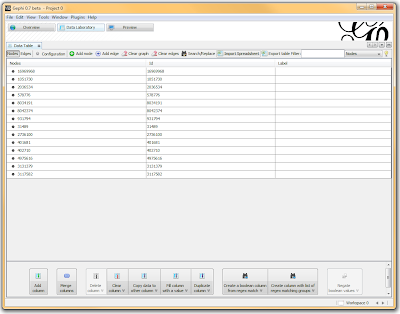
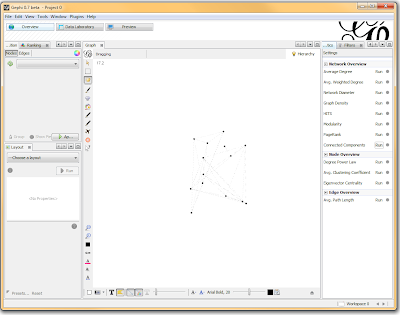
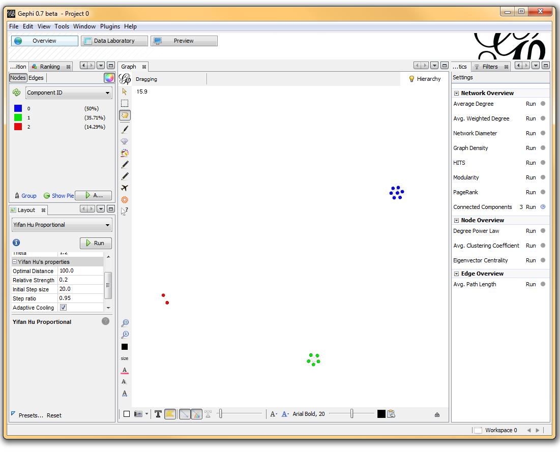
Once loaded, I clicked on the “Overview” tab and I can see my graph. The graph looks like a big mess, but we don’t really care how it looks – we’re going to run an analysis. In the “statistics” tab on the right-hand side, you’ll see an option for “connected components”. This runs an algorithm that picks apart and labels collections of nodes that are connected. Running this only takes a second.
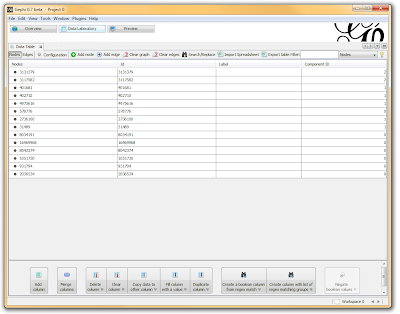
I then click on the “Data Laboratory” tab again, and I can see that my nodes are labeled with an ID. This corresponds to the Locus those SNPs represent.
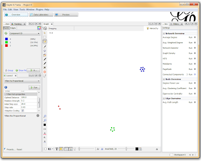
If you want to actually SEE how these relationships fall out, we’ll need to run a layout engine. Back on the “Overview” tab, on the lower left-hand side, there is a drop-down allowing you to choose a layout engine. I have found YifanHu’s Multilevel to be the quickest and most effective for separating small groups like these. Depending on the size of your graph, it may take a moment to run. Once its finished, you should be able to see the components clearly separated. If you want, you can color code them by clicking the green “refresh” button in the “partition” tab in the upper left corner. This reloads the drop-down menu and will provide you with an option to color the nodes by component ID. Select this, and click apply to see the results!
I’ve used Gephi component analysis to do all kinds of fun things, like the number of families in a study using pairwise IBD estimates, looking at patterns of phenotype sharing in pedigrees, and even visualizing citation networks. Sometimes representing a problem as a graph lets you find patterns more easily than examining tables of numbers.
Recently, some collaborators from the PAGE study had a list of a few hundred SNPs gathered from multiple loci across the genome. For analysis purposes, they were interested in quantifying the number of loci these SNPs represented – in other words, how many distinct signals were represented by their collection of SNPs.
We had linkage disequilibrium data from the HapMap for all pairs of SNPs, and we filtered this using an r-squared cutoff. What we were left with was a mess of SNP pairs that could be tedious to sort through in a spreadsheet. Instead, I represented each pair of SNPs as an edge in a network and loaded the data into Gephi, which provides some wonderful analysis tools. Suppose my LD data is structured like this:
| SNP1 | SNP2 | d-prime | r-squared |
| 16969968 | 1051730 | 0.98 | 1 |
| 2036534 | 1051730 | 0.92 | 0.205 |
| 578776 | 1051730 | 0.96 | 0.23 |
| 8034191 | 1051730 | 1 | 0.961 |
| 8042374 | 1051730 | 0.99 | 0.205 |
| ... | ... | ... | ... |
In a spreadsheet application, I sorted and filtered the LD pairings I wanted using either the r-squared or the d-prime columns. I then deleted any rows that didn’t meet my cutoff, renamed the header for SNP1 to “Source” and SNP2 to “Target”, and exported the file as a comma-separated file (.csv). I opened Gephi, clicked the “Data Laboratory” tab, and Import Spreadsheet to load my data.

Once loaded, I clicked on the “Overview” tab and I can see my graph. The graph looks like a big mess, but we don’t really care how it looks – we’re going to run an analysis. In the “statistics” tab on the right-hand side, you’ll see an option for “connected components”. This runs an algorithm that picks apart and labels collections of nodes that are connected. Running this only takes a second.

I then click on the “Data Laboratory” tab again, and I can see that my nodes are labeled with an ID. This corresponds to the Locus those SNPs represent.

If you want to actually SEE how these relationships fall out, we’ll need to run a layout engine. Back on the “Overview” tab, on the lower left-hand side, there is a drop-down allowing you to choose a layout engine. I have found YifanHu’s Multilevel to be the quickest and most effective for separating small groups like these. Depending on the size of your graph, it may take a moment to run. Once its finished, you should be able to see the components clearly separated. If you want, you can color code them by clicking the green “refresh” button in the “partition” tab in the upper left corner. This reloads the drop-down menu and will provide you with an option to color the nodes by component ID. Select this, and click apply to see the results!
I’ve used Gephi component analysis to do all kinds of fun things, like the number of families in a study using pairwise IBD estimates, looking at patterns of phenotype sharing in pedigrees, and even visualizing citation networks. Sometimes representing a problem as a graph lets you find patterns more easily than examining tables of numbers.
Thursday, September 8, 2011
I'm Starting a New Position at the University of Virginia
I just accepted an offer for a faculty position at the University of Virginia in the Center for Public Health Genomics / Department of Public Health Sciences. Starting in October I will be developing and directing a new centralized bioinformatics core in the UVA School of Medicine. Over the next few weeks I'm taking a much-needed vacation next door in Kauai and then packing up for the move to Charlottesville. Posts here may be sparse over the next few weeks, but once I start my new gig I'll be sure to make up for it. And if you're bioinformatics-savvy and in the job market keep an eye out here - once I figure out what I need I will soon be hiring, and will repost any job announcements here.
I've enjoyed my postdoc here at the University of Hawaii Cancer Center, and there is much I'll miss about island life out here in the Pacific. But I'm very seriously looking forward to getting started in this wonderful opportunity at UVA. Thank you all for your comments, suggestions, and help when I needed it. I'll be back online in a few weeks - until then, follow me on Twitter (@genetics_blog).
Aloha!
True Hypotheses are True, False Hypotheses are False
I just read Gregory Cooper and Jay Shendure's review "Needles in stacks of needles: finding disease-causal variants in a wealth of genomic data" in Nature Reviews Genetics. It's a good review about how to narrow down deleterious disease-causing variants from many, many variants throughout the genome when statistics and genetic information alone isn't enough.
I really liked how they framed the multiple-testing problem that routinely plagues large-scale genetic studies, where nominal significance thresholds can yield many false positives when applied to multiple hypothesis tests:
Check out the full review at Nature Reviews Genetics:
Needles in stacks of needles: finding disease-causal variants in a wealth of genomic data
I really liked how they framed the multiple-testing problem that routinely plagues large-scale genetic studies, where nominal significance thresholds can yield many false positives when applied to multiple hypothesis tests:
However, true hypotheses are true, and false hypotheses are false, regardless of how many are tested. As such, the actual 'multiple testing burden' depends on the proportion of true and false hypotheses in any given set: that is, the 'prior probability' that any given hypothesis is true, rather than the number of tests per se. This challenge can thus be viewed as a 'naive hypothesis testing' problem — that is, when in reality only one or a few variants are causal for a given phenotype, but all (or many) variants are a priori equally likely candidates, the prior probability of any given variant being causal is miniscule. As a consequence, extremely convincing data are required to support causality, which is potentially unachievable for some true positives.
Defining the challenge in terms of hypothesis quality rather than quantity, however, points to a solution. Specifically, experimental or computational approaches that provide assessments of variant function can be used to better estimate the prior probability that any given variant is phenotypically important, and these approaches thereby boost discovery power.
Check out the full review at Nature Reviews Genetics:
Needles in stacks of needles: finding disease-causal variants in a wealth of genomic data
Wednesday, September 7, 2011
Excel Template for Mapping Four 96-Well Plates to One 384-Well Plate
Daniel Cook in Jeff Murray's lab at the University of Iowa put together this handy Excel template for keeping track of how samples from four 96-well plates are interleaved to configure a single 384-well plate using robotic liquid handling systems, like the Hydra II.
Paste in lists of samples on your 96-well plates:

And you'll get out a map of how the 384-well plate layout:

And a summary list:

You can download the Excel file here. Thanks for sharing, Daniel.
Paste in lists of samples on your 96-well plates:
And you'll get out a map of how the 384-well plate layout:

And a summary list:

You can download the Excel file here. Thanks for sharing, Daniel.
Wednesday, August 31, 2011
Personal Genomics and Data Sharing Survey
I was recently contacted by a couple of German biologists working on a project evaluating opinions on sharing raw data from DTC genetic testing companies like 23andme. A handful of people like the gang at Genomes Unzipped, the PGP-10, and others at SNPedia have released their own genotype or sequencing data into the public domain. As of now, data like this is scattered around the web and most of it is not attached to any phenotype data.
These three biologists are working on a website that collects genetic data as well as phenotypic data. The hope is to make it easy to find and access appropriate data and to become a resource for a kind of open-source GWAS - similar to the research 23andMe performs in its walled garden right now.
But because of privacy concerns, many people (myself included) hesitate to freely publish their genetic data for the world to see. These three biologists are conducting a survey to assess how willing people might be to participate in something like this, and for what reasons they would (or would not). The survey can be accessed at http://bit.ly/genotyping_survey. It took about 2 minutes for me to complete, and you can optionally sign up to receive an email with their results once they've completed the survey.
Although I'm still hesitant to participate in something like this myself, I like the idea, and I'm very interested to see the results of their survey. Hit the link below if you'd like to take the quick survey.
Personal Genomics and Data Sharing Survey
Monday, August 29, 2011
Bioinformatics Posters Collection
I mentioned BioStar in a previous post about getting all your questions answered. I can't emphasize enough how helpful the BioStar and other StackExchange communities are. Whenever I ask a statistics question on CrossValidated or a programming question on StackOverflow I often multiple answers within 10 minutes.
Recently there was a question on BioStar from someone making their poster for a bioinformatics poster presentation and wanted some inspiration for design and layout. No less than 7 community members posted responses the same day, linking to sites where you can download poster presentations, including VIZBI 2011 (workshop on visualizing biological data), F1000 Posters (which collects posters from the Intelligent Systems for Molecular Biology conference), Nature Precedings (not specifically limited to bioinformatics), and several others.
While you can see plenty of posters at the meeting you're attending, it isn't much help when you're trying to design and layout your poster beforehand. I've used the same tired old template for poster presentations for years, and it's helpful to see examples of other bioinformatics posters for fresh ideas about design and layout.
I would also encourage you to deposit some of your posters in places like F1000 (deposit link) or Nature Precedings (submission link). While these aren't peer-reviewed, it can really increase the visibility of your work, and it gives you a permanent DOI (at least for Nature Precedings) that you can link to or reference in other scientific communication.
See this Q&A at BioStar for more.
Monday, August 22, 2011
Estimating Trait Heritability from GWAS Data
Peter Visscher and colleagues have recently published a flurry of papers employing a new software package called GCTA to estimate the heritability of traits using GWAS data (GCTA stands for Genome-wide Complex Trait Analysis -- clever acronymity!). The tool, supported (and presumably coded) by Jian Yang is remarkably easy to use, based in part on the familiar PLINK commandline interface. The GCTA Homepage provides an excellent walk-through of the available options.
The basic idea is to use GWAS data to estimate the degree of "genetic sharing" or relatedness among the samples, computing what the authors call a genetic relationship matrix (GRM). The degree of genetic sharing among samples is then related to the amount of phenotypic sharing using restricted maximum likelihood analysis (REML). The result is an estimate of the variance explained by the SNPs used to generate the GRM. Full details of the stats along with all the gory matrix notation can be found in their software publication.
The approach has been applied to several disorders studied by the WTCCC and to a recent study of human height. Interestingly, the developers have also used the approach to partition the trait variance across chromosomes, resulting in something similar to population-based variance-components linkage analysis. The approach works for both quantitative and dichotomous traits, however the authors warn that variance estimates of dichotomous trait liability are influenced by genotyping artifacts.
The package also includes several other handy features, including a relatively easy way to estimate principal components for population structure correction, a GWAS simulation tool, and a regression-based LD mapping tool. Download and play -- a binary is available for Linux, MacOS, and DOS/Windows.
Monday, August 15, 2011
Sync Your Rprofile Across Multiple R Installations
Your Rprofile is a script that R executes every time you launch an R session. You can use it to automatically load packages, set your working directory, set options, define useful functions, and set up database connections, and run any other code you want every time you start R.
If you're using R in Linux, it's a hidden file in your home directory called ~/.Rprofile, and if you're on Windows, it's usually in the program files directory: C:\Program Files\R\R-2.12.2\library\base\R\Rprofile. I sync my Rprofile across several machines and operating systems by creating a separate script called called syncprofile.R and storing this in my Dropbox. Then, on each machine, I edit the real Rprofile to source the syncprofile.R script that resides in my Dropbox.
One of the disadvantages of doing this, however, is that all the functions you define and variables you create are sourced into the global environment (.GlobalEnv). This can clutter your workspace, and if you want to start clean using rm(list=ls(all=TRUE)), you'll have to re-source your syncprofile.R script every time.
It's easy to get around this problem. Rather than simply appending source(/path/to/dropbox/syncprofile.R) to the end of your actual Rprofile, first create a new environment, source that script into that new environment, and attach that new environment. So you'll add this to the end of your real Rprofile on each machine/installation:
All the functions and variables you've defined are now available but they no longer clutter up the global environment.
If you have code that you only want to run on specific machines, you can still put that into each installation's Rprofile rather than the syncprofile.R script that you sync using Dropbox. Here's what my syncprofile.R script looks like - feel free to take whatever looks useful to you.
If you're using R in Linux, it's a hidden file in your home directory called ~/.Rprofile, and if you're on Windows, it's usually in the program files directory: C:\Program Files\R\R-2.12.2\library\base\R\Rprofile. I sync my Rprofile across several machines and operating systems by creating a separate script called called syncprofile.R and storing this in my Dropbox. Then, on each machine, I edit the real Rprofile to source the syncprofile.R script that resides in my Dropbox.
One of the disadvantages of doing this, however, is that all the functions you define and variables you create are sourced into the global environment (.GlobalEnv). This can clutter your workspace, and if you want to start clean using rm(list=ls(all=TRUE)), you'll have to re-source your syncprofile.R script every time.
It's easy to get around this problem. Rather than simply appending source(/path/to/dropbox/syncprofile.R) to the end of your actual Rprofile, first create a new environment, source that script into that new environment, and attach that new environment. So you'll add this to the end of your real Rprofile on each machine/installation:
my.env <- new.env()
sys.source("C:/Users/st/Dropbox/R/Rprofile.r", my.env)
attach(my.env)
All the functions and variables you've defined are now available but they no longer clutter up the global environment.
If you have code that you only want to run on specific machines, you can still put that into each installation's Rprofile rather than the syncprofile.R script that you sync using Dropbox. Here's what my syncprofile.R script looks like - feel free to take whatever looks useful to you.
Friday, August 5, 2011
Friday Links: R, OpenHelix Bioinformatics Tips, 23andMe, Perl, Python, Next-Gen Sequencing
I haven't posted much here recently, but here is a roundup of a few of the links I've shared on Twitter (@genetics_blog) over the last two weeks.
Here is a nice tutorial on accessing high-throughput public data (from NCBI) using R and Bioconductor.
Cloudnumbers.com, a startup that allows you to run high-performance computing (HPC) applications in the cloud, now supports the previously mentioned R IDE, RStudio.
23andMe announced a project to enroll 10,000 African-Americans for research by giving participants their personal genome service for free. You can read about it here at 23andMe or here at Genetic Future.
Speaking of 23andMe, they emailed me a coupon code (8WR9U9) for getting $50 off their personal genome service, making it $49 instead of $99. Not sure how long it will last.
I previously took a poll which showed that most of you use Mendeley to manage your references. Mendeley recently released version 1.0, which includes some nice features like duplicate detection, better library organization (subfolders!), and a better file organization tool. You can download it here.
An interesting blog post by Michael Barton on how training and experience in bioinformatics leads to a wide set of transferable skills.
Dienekes releases a free DIY admixture program to analyze genomic ancestry.
A few tips from OpenHelix: the new SIB Bioinformatics Resource Portal, and testing correlation between SNPs and gene expression using SNPexp.
A nice animation describing a Circos plot from PacBio's E. coli paper in NEJM.
The Court of Appeals for the Federal Circuit reversed the lower court's invalidation of Myriad Genetics' patents on BRCA1/2, reinstating most of the claims in full force. Thoughtful analysis from Dan Vorhaus here.
Using the Linux shell and perl to delete files in the current directory that don't contain the right number of lines: If you want to get rid of all files in the current directory that don't have exactly 42 lines, run this code at the command line (*be very careful with this one!*): for f in *.txt;do perl -ne 'END{unlink $ARGV unless $.==42}' ${f} ;done
The previously mentioned Hitchhiker's Guide to Next-Generation Sequencing by Gabe Rudy at Golden Helix is now available in PDF format here. You can also find the related post describing all the various file formats used in NGS in PDF format here.
The Washington Post ran an article about the Khan Academy (http://www.khanacademy.org/), which has thousands of free video lectures, mostly on math. There are also a few computer science lectures that teach Python programming. (Salman Khan also appeared on the Colbert Report a few months ago).
Finally, I stumbled across this old question on BioStar with lots of answers about methods for short read mapping with next-generation sequencing data.
...
And here are a few interesting papers I shared:
Nature Biotechnology: Structural variation in two human genomes mapped at single-nucleotide resolution by whole genome de novo assembly
PLoS Genetics: Gene-Based Tests of Association
PLoS Genetics: Fine Mapping of Five Loci Associated with Low-Density Lipoprotein Cholesterol Detects Variants That Double the Explained Heritability
Nature Reviews Genetics: Systems-biology approaches for predicting genomic evolution
Genome Research: A comprehensively molecular haplotype-resolved genome of a European individual (paper about the importance of phase in genetic studies)
Nature Reviews Microbiology: Unravelling the effects of the environment and host genotype on the gut microbiome.
...
Monday, July 25, 2011
Scatterplot matrices in R
I just discovered a handy function in R to produce a scatterplot matrix of selected variables in a dataset. The base graphics function is pairs(). Producing these plots can be helpful in exploring your data, especially using the second method below.
Try it out on the built in iris dataset. (data set gives the measurements in cm of the variables sepal length and width and petal length and width, respectively, for 50 flowers from each of 3 species of iris. The species are Iris setosa, versicolor, and virginica).
 Looking at the pairs help page I found that there's another built-in function, panel.smooth(), that can be used to plot a loess curve for each plot in a scatterplot matrix. Pass this function to the lower.panel argument of the pairs function. The panel.cor() function below can compute the absolute correlation between pairs of variables, and display these in the upper panels, with the font size proportional to the absolute value of the correlation.

Finally, you can produce a similar plot using ggplot2, with the diagonal showing the kernel density.

See more on the pairs function here.
...
Update: A tip of the hat to Hadley Wickham (@hadleywickham) for pointing out two packages useful for scatterplot matrices. The gpairs package has some useful functionality for showing the relationship between both continuous and categorical variables in a dataset, and the GGally package extends ggplot2 for plot matrices.
Try it out on the built in iris dataset. (data set gives the measurements in cm of the variables sepal length and width and petal length and width, respectively, for 50 flowers from each of 3 species of iris. The species are Iris setosa, versicolor, and virginica).
# panel.smooth function is built in.
# panel.cor puts correlation in upper panels, size proportional to correlation
panel.cor <- function(x, y, digits=2, prefix="", cex.cor, ...)
{
    usr <- par("usr"); on.exit(par(usr))
    par(usr = c(0, 1, 0, 1))
    r <- abs(cor(x, y))
    txt <- format(c(r, 0.123456789), digits=digits)[1]
    txt <- paste(prefix, txt, sep="")
    if(missing(cex.cor)) cex.cor <- 0.8/strwidth(txt)
    text(0.5, 0.5, txt, cex = cex.cor * r)
}

# Plot #2: same as above, but add loess smoother in lower and correlation in upper
pairs(~Sepal.Length+Sepal.Width+Petal.Length+Petal.Width, data=iris,
      lower.panel=panel.smooth, upper.panel=panel.cor,
      pch=20, main="Iris Scatterplot Matrix")
Finally, you can produce a similar plot using ggplot2, with the diagonal showing the kernel density.
# Plot #3: similar plot using ggplot2
# install.packages("ggplot2") ## uncomment to install ggplot2
library(ggplot2)
plotmatrix(with(iris, data.frame(Sepal.Length, Sepal.Width, Petal.Length, Petal.Width)))
See more on the pairs function here.
...
Update: A tip of the hat to Hadley Wickham (@hadleywickham) for pointing out two packages useful for scatterplot matrices. The gpairs package has some useful functionality for showing the relationship between both continuous and categorical variables in a dataset, and the GGally package extends ggplot2 for plot matrices.
Tuesday, July 12, 2011
Download 69 Complete Human Genomes
Sequencing company Complete Genomics recently made available 69 ethnically diverse complete human genome sequences: a Yoruba trio; a Puerto Rican trio; a 17-member, 3-generation pedigree; and a diversity panel representing 9 different populations. Some of the samples partially overlap with HapMap and the 1000 Genomes Project. The data can be downloaded directly from the FTP site. See the link below for more details on the directory contents, and have a look at the quick start guide to working with complete genomics data.
Complete Genomics - Sample Human Genome Sequence Data
Complete Genomics - Sample Human Genome Sequence Data
Thursday, June 30, 2011
Mapping SNPs to Genes for GWAS Enrichment Analysis
There are several tools available for conducting a post-hoc analysis of GWAS data looking for enrichment of significant SNPs using literature or pathway based resources. Examples include GRAIL, ALLIGATOR, and WebGestalt among others (see SNPath R Package). Since gene enrichment and pathway analysis essentially evolved from methods for analyzing gene expression data, many of these tools require specific gene identifiers as input.
To prep GWAS data for analyses such as these, you'll need to ensure that your SNPs have current map position information, and assign each SNP to genes. To update your map information, the easiest resource to use is the UCSC Tables browser.
To use UCSC, go to the TABLES link on the browser page. Select the current assembly, "Variation and Repeats" for group, "Common SNPs(132)" for the track, and "snp132Commmon" for the table. Now you'll need to upload your SNP list. You can manually edit the map file using a tool like Excel or Linux commands like awk to extract the rs_ids for your SNPs into a text file. Upload this file by clicking the "Upload List" button in the "identifiers" section. Once this file has uploaded, select "BED - browser extensible data" for the output format and click "Get Output". The interface will ask you if you want to add upstream or downstream regions -- for SNPs this makes little sense, so leave these at zero. Also, ensure that "Send to Galaxy" is not checked.
This will export a BED file containing the positions of all your SNPs in the build you selected, preferably the most current one -- let's call it SNPs.bed. BED files were developed by the folks behind the UCSC browser to document genomic annotations. The basic format is:
Because BED files were designed to list genomic ranges, SNPs are listed with a range of 1 BP, meaning the StartPosition is the location of the SNP and the EndPosition is the location of the SNP + 1.
The next step is to map these over to genes. To save a lot of effort resolving identifiers (which is no fun, I promise), I have generated a list of ~17,000 genes that are consistently annotated across Ensembl and Entrez-gene databases, and which have HUGO identifiers. These files are available here:
The genes listed in these files were generated by comparing the cross-references between the Ensembl and Entrez-gene databases. To arrive at a set of "consensus" genes, I selected only genes where Ensembl refers to an Entrez-gene with the same coordinates, and that Entrez-gene entry refers back to the same Ensembl gene. Nearly all cases of inconsistent cross-referencing are genes annotated based on electronic predictions, or genes with multiple or inconsistent mappings. For the purpose of doing enrichment analysis, these would be ignored anyway, as they aren't likely to show up in pathway or functional databases. For these genes, we then obtained the HUGO approved gene identifier. The coordinates for all genes are mapped using hg19/GRChB37.
BED files are plain text and easy to modify. If you wanted to add 10KB to the gene bounds, for example, you could alter these files using excel formulas, or with a simple awk command:
You'll need to download a collection of utilities called http://www.blogger.com/img/blank.gif BEDTools. If you have access to a Linux system, this should be fairly straightforward. These utilities are already installed on Vanderbilt's Linux application servers, but to compile the program yourself, download the .tar.gz file above, and use the following commands to compile:
tar -zxvf BEDTools..tar.gz
cd BEDTools
make clean
make all
ls bin
# copy the binaries to a directory in your PATH. e.g.,
sudo cp bin/* /usr/local/bin
Once you get BEDTools installed, there is a utility called intersectBed. This command allows you to examine the overlap of two BED files. Since we have our collection of SNPs and our collections of Genes in BED file format already, all we need to do is run the command.
This will print to the screen any SNP that falls within an EntrezGene boundary, along with the coordinates from each entry in each file. To strip this down to only RS numbers and gene identifiers, we can pipe this through awk.
This will produce a tab-delimited file with SNPs that fall within genes identified by EntrezGene ID number. For HUGO names or Ensembl gene IDs, use the corresponding BED file.
To prep GWAS data for analyses such as these, you'll need to ensure that your SNPs have current map position information, and assign each SNP to genes. To update your map information, the easiest resource to use is the UCSC Tables browser.
To use UCSC, go to the TABLES link on the browser page. Select the current assembly, "Variation and Repeats" for group, "Common SNPs(132)" for the track, and "snp132Commmon" for the table. Now you'll need to upload your SNP list. You can manually edit the map file using a tool like Excel or Linux commands like awk to extract the rs_ids for your SNPs into a text file. Upload this file by clicking the "Upload List" button in the "identifiers" section. Once this file has uploaded, select "BED - browser extensible data" for the output format and click "Get Output". The interface will ask you if you want to add upstream or downstream regions -- for SNPs this makes little sense, so leave these at zero. Also, ensure that "Send to Galaxy" is not checked.
This will export a BED file containing the positions of all your SNPs in the build you selected, preferably the most current one -- let's call it SNPs.bed. BED files were developed by the folks behind the UCSC browser to document genomic annotations. The basic format is:
Chromosome|StartPosition|EndPosition|FeatureLabel
Because BED files were designed to list genomic ranges, SNPs are listed with a range of 1 BP, meaning the StartPosition is the location of the SNP and the EndPosition is the location of the SNP + 1.
The next step is to map these over to genes. To save a lot of effort resolving identifiers (which is no fun, I promise), I have generated a list of ~17,000 genes that are consistently annotated across Ensembl and Entrez-gene databases, and which have HUGO identifiers. These files are available here:
Hugo Genes
Entrez Genes
Ensembl Genes
The genes listed in these files were generated by comparing the cross-references between the Ensembl and Entrez-gene databases. To arrive at a set of "consensus" genes, I selected only genes where Ensembl refers to an Entrez-gene with the same coordinates, and that Entrez-gene entry refers back to the same Ensembl gene. Nearly all cases of inconsistent cross-referencing are genes annotated based on electronic predictions, or genes with multiple or inconsistent mappings. For the purpose of doing enrichment analysis, these would be ignored anyway, as they aren't likely to show up in pathway or functional databases. For these genes, we then obtained the HUGO approved gene identifier. The coordinates for all genes are mapped using hg19/GRChB37.
BED files are plain text and easy to modify. If you wanted to add 10KB to the gene bounds, for example, you could alter these files using excel formulas, or with a simple awk command:
awk '{printf("%d\t%d\t%d\t%s\n", $1, $2-10000, $3+10000, $4); }' ensemblgenes.bed
You'll need to download a collection of utilities called http://www.blogger.com/img/blank.gif BEDTools. If you have access to a Linux system, this should be fairly straightforward. These utilities are already installed on Vanderbilt's Linux application servers, but to compile the program yourself, download the .tar.gz file above, and use the following commands to compile:
cd BEDTools
make clean
make all
ls bin
# copy the binaries to a directory in your PATH. e.g.,
sudo cp bin/* /usr/local/bin
Once you get BEDTools installed, there is a utility called intersectBed. This command allows you to examine the overlap of two BED files. Since we have our collection of SNPs and our collections of Genes in BED file format already, all we need to do is run the command.
intersectBed -a SNPs.bed -b entrezgenes.bed -wa -wb
This will print to the screen any SNP that falls within an EntrezGene boundary, along with the coordinates from each entry in each file. To strip this down to only RS numbers and gene identifiers, we can pipe this through awk.
intersectBed -a SNPs.bed -b entrezgenes.bed -wa -wb | awk '{printf("%s\t%s\n", $4, $8);}'
This will produce a tab-delimited file with SNPs that fall within genes identified by EntrezGene ID number. For HUGO names or Ensembl gene IDs, use the corresponding BED file.
Wednesday, June 29, 2011
Nucleic Acids Research Web Server Issue
Nucleic Acids Research just published its Web Server Issue, featuring new and updates to existing web servers and applications for genomics and proteomics research. In case you missed it, be sure to check out the Database Issue that came out earlier this year.
This web server issue has lots of papers on tools for microRNA analysis, and protein/RNA secondary structure analysis and annotation. Here are a few that sounded interesting for those doing systems genomics and trying to put findings into a functional, biologically relevant context:
g:Profiler—a web server for functional interpretation of gene lists (2011 update)
Abstract: Functional interpretation of candidate gene lists is an essential task in modern biomedical research. Here, we present the 2011 update of g:Profiler (http://biit.cs.ut.ee/gprofiler/), a popular collection of web tools for functional analysis. g:GOSt and g:Cocoa combine comprehensive methods for interpreting gene lists, ordered lists and list collections in the context of biomedical ontologies, pathways, transcription factor and microRNA regulatory motifs and protein–protein interactions. Additional tools, namely the biomolecule ID mapping service (g:Convert), gene expression similarity searcher (g:Sorter) and gene homology searcher (g:Orth) provide numerous ways for further analysis and interpretation. In this update, we have implemented several features of interest to the community: (i) functional analysis of single nucleotide polymorphisms and other DNA polymorphisms is supported by chromosomal queries; (ii) network analysis identifies enriched protein–protein interaction modules in gene lists; (iii) functional analysis covers human disease genes; and (iv) improved statistics and filtering provide more concise results. g:Profiler is a regularly updated resource that is available for a wide range of species, including mammals, plants, fungi and insects.
KOBAS 2.0: a web server for annotation and identification of enriched pathways and diseases
Abstract: High-throughput experimental technologies often identify dozens to hundreds of genes related to, or changed in, a biological or pathological process. From these genes one wants to identify biological pathways that may be involved and diseases that may be implicated. Here, we report a web server, KOBAS 2.0, which annotates an input set of genes with putative pathways and disease relationships based on mapping to genes with known annotations. It allows for both ID mapping and cross-species sequence similarity mapping. It then performs statistical tests to identify statistically significantly enriched pathways and diseases. KOBAS 2.0 incorporates knowledge across 1327 species from 5 pathway databases (KEGG PATHWAY, PID, BioCyc, Reactome and Panther) and 5 human disease databases (OMIM, KEGG DISEASE, FunDO, GAD and NHGRI GWAS Catalog). KOBAS 2.0 can be accessed at http://kobas.cbi.pku.edu.cn.
ICSNPathway: identify candidate causal SNPs and pathways from genome-wide association study by one analytical framework
Abstract: Genome-wide association study (GWAS) is widely utilized to identify genes involved in human complex disease or some other trait. One key challenge for GWAS data interpretation is to identify causal SNPs and provide profound evidence on how they affect the trait. Currently, researches are focusing on identification of candidate causal variants from the most significant SNPs of GWAS, while there is lack of support on biological mechanisms as represented by pathways. Although pathway-based analysis (PBA) has been designed to identify disease-related pathways by analyzing the full list of SNPs from GWAS, it does not emphasize on interpreting causal SNPs. To our knowledge, so far there is no web server available to solve the challenge for GWAS data interpretation within one analytical framework. ICSNPathway is developed to identify candidate causal SNPs and their corresponding candidate causal pathways from GWAS by integrating linkage disequilibrium (LD) analysis, functional SNP annotation and PBA. ICSNPathway provides a feasible solution to bridge the gap between GWAS and disease mechanism study by generating hypothesis of SNP → gene → pathway(s). The ICSNPathway server is freely available at http://icsnpathway.psych.ac.cn/.
AnnotQTL: a new tool to gather functional and comparative information on a genomic region
Abstract: AnnotQTL is a web tool designed to aggregate functional annotations from different prominent web sites by minimizing the redundancy of information. Although thousands of QTL regions have been identified in livestock species, most of them are large and contain many genes. This tool was therefore designed to assist the characterization of genes in a QTL interval region as a step towards selecting the best candidate genes. It localizes the gene to a specific region (using NCBI and Ensembl data) and adds the functional annotations available from other databases (Gene Ontology, Mammalian Phenotype, HGNC and Pubmed). Both human genome and mouse genome can be aligned with the studied region to detect synteny and segment conservation, which is useful for running inter-species comparisons of QTL locations. Finally, custom marker lists can be included in the results display to select the genes that are closest to your most significant markers. We use examples to demonstrate that in just a couple of hours, AnnotQTL is able to identify all the genes located in regions identified by a full genome scan, with some highlighted based on both location and function, thus considerably increasing the chances of finding good candidate genes. AnnotQTL is available at http://annotqtl.genouest.org.
Génie: literature-based gene prioritization at multi genomic scale
Abstract: Biomedical literature is traditionally used as a way to inform scientists of the relevance of genes in relation to a research topic. However many genes, especially from poorly studied organisms, are not discussed in the literature. Moreover, a manual and comprehensive summarization of the literature attached to the genes of an organism is in general impossible due to the high number of genes and abstracts involved. We introduce the novel Génie algorithm that overcomes these problems by evaluating the literature attached to all genes in a genome and to their orthologs according to a selected topic. Génie showed high precision (up to 100%) and the best performance in comparison to other algorithms in most of the benchmarks, especially when high sensitivity was required. Moreover, the prioritization of zebrafish genes involved in heart development, using human and mouse orthologs, showed high enrichment in differentially expressed genes from microarray experiments. The Génie web server supports hundreds of species, millions of genes and offers novel functionalities. Common run times below a minute, even when analyzing the human genome with hundreds of thousands of literature records, allows the use of Génie in routine lab work. Availability: http://cbdm.mdc-berlin.de/tools/genie/.
Nucleic Acids Research: Web Server Issue
Wednesday, June 22, 2011
Steal This Blog!

Tuesday, June 14, 2011
Displaying Regression Coefficients from Complex Analyses
Genome-wide association studies have produced a wealth of new genetic associations to numerous traits over the last few years. As such, new studies of these phenotypes often attempt to replicate previous associations in their samples, or examine how the effects of these SNPs are altered by environmental factors or clinical subtypes. This growing trend means that the results section must become multi-dimensional, accounting for all the ways by which samples were partitioned for analysis.
A great way to display regression coefficients is with forest plots, and an excellent example can be seen in the previous post.
There are various ways to produce these useful plots, but our colleague Sarah Pendergrass recently published a very nice tool for creating high-dimensional forest plots, like the one seen below.

This tool, called Synthesis-View provides several additional plot types that make the results of complex analyses much more accessible. You can read about the details here.
While Sarah designed this for the examination of multi-ethnic cohort studies, it could easily be adapted to simultaneously plot coefficients stratified by sex, age groups, or clinical subtypes.
Tuesday, June 7, 2011
Replication of >180 Genetic Associations with Self-Report Medical Data
DNA genotyping and sequencing are getting cheaper every day. As Oxford Nanopore CTO Clive Brown recently discussed at Genomes Unzipped, when the cost of a full DNA sequence begins to fall below $1000, the value of having that information far outweighs the cost of data generation.
Participant collection and ascertainment, however, isn't getting cheaper any time soon, spurring a burgeoning interest in using DNA biobanks and electronic medical records (EMRs) for genomics research (reviewed here). In fact, this is exactly the focus of the eMERGE network - a consortium of five sites having biobanks linked to electronic medical records for genetic research. The first order of business for the eMERGE network was assessment - can DNA biobanks + EMRs be used for genetic research? This question was answered with a demonstration project using Vanderbilt University's BioVU biobank+EMR. Here, 21 previously reported associations to five complex diseases were tested for association to electronically abstracted phenotypes from BioVU's EMR. This forest plot shows that for the 21 previously reported associations (red), five replicated at a nominal significance threshold, and for the rest, the calculated odds ratios (blue) trended in the same direction as the reported association.

While electronic phenotyping is much cheaper than ascertainment in the traditional sense, it can still be costly and labor intensive, involving interative cycles of manual medical record chart review followed by refinement of natural language processing algorithms. In many instances, self-report can be comparably accurate, and much easier to obtain (for example, compare the eMERGE network's hypothyroidism phenotyping algorithm with simply asking the question: "Have you ever been diagnosed with Hashmoto's Thyroiditis?").
This is the approach to genetic research 23andMe is taking. Joyce Tung presented some preliminary results at last year's ASHG conference, and now you can read the preprint of the research paper online at Nature Preceedings - "Efficient Replication of Over 180 Genetic Associations with Self-Reported Medical Data". In this paper the authors amassed self-reported data from >20,000 genotyped 23andMe customers on 50 medical phenotypes and attempted to replicate known findings from the GWAS catalog. Using only self-reported data, the authors were able to replicate at a nominal significance level 75% of the previously reported associations that they were powered to detect. Figure 1 from the preprint is similar to the figure above, where blue X's are prior GWAS hits and black dots and lines represent their ORs and 95% CI's:

One might ask whether there is any confounding due to the fact that 23andMe customers can view trait/disease risks before answering questions (see this paper and this discussion by Luke Jostins). The authors investigated this and did not observe a consistent or significant effect of seeing genetic risk results before answering questions. There's also a good discussion regarding SNPs that failed to replicate, and a general discussion of using self-report from a recontactable genotyped cohort for genetic studies.
Other than 23andMe's customer base, I can't think of any other genotyped, recontactable cohort that have incentive to fill out research surveys for this kind of study. But this team has shown here and in the past that this model for performing genetic research works and is substantially cheaper than traditional ascertainment or even mining electronic medical records. I look forward to seeing more research results from this group!
Efficient Replication of Over 180 Genetic Associations with Self-Reported Medical Data
Subscribe to:
Posts (Atom)
