Getting Genetics Done 2012 In Review

Here are links to all of this year's posts (excluding seminar/webinar announcements), with the most visited posts in bold italic. As always, you can follow me on Twitter for more frequent updates. Happy new year!

New Year's Resolution: Learn How to Code

Annotating limma Results with Gene Names for Affy Microarrays

Your Publications (with PMCID) as a PubMed Query

Pathway Analysis for High-Throughput Genomics Studies

find | xargs ... Like a Boss

Redesign by Subtraction

Video Tip: Convert Gene IDs with Biomart

RNA-Seq Methods & March Twitter Roundup

Awk Command to Count Total, Unique, and the Most Abundant Read in a FASTQ file

Video Tip: Use Ensembl BioMart to Quickly Get Ortholog Information

Stepping Outside My Open-Source Comfort Zone: A First Look at Golden Helix SVS

How to Stay Current in Bioinformatics/Genomics

The HaploREG Database for Functional Annotation of SNPs

Identifying Pathogens in Sequencing Data

Browsing dbGAP Results

Fix Overplotting with Colored Contour Lines

Plotting the Frequency of Twitter Hashtag Usage Over Time with R and ggplot2

Cscan: Finding Gene Expression Regulators with ENCODE ChIP-Seq Data

More on Exploring Correlations in R

DESeq vs edgeR Comparison

Learn R and Python, and Have Fun Doing It

STAR: ultrafast universal RNA-seq aligner

RegulomeDB: Identify DNA Features and Regulatory Elements in Non-Coding Regions

Copy Text to the Local Clipboard from a Remote SSH Session

Differential Isoform Expression With RNA-Seq: Are We Really There Yet?

Differential Isoform Expression With RNA-Seq: Are We Really There Yet?

In case you missed it, a new paper was published in Nature Biotechnology on a method for detecting isoform-level differential expression with RNA-seq Data:

Trapnell, Cole, et al. "Differential analysis of gene regulation at transcript resolution with RNA-seq." Nature Biotechnology (2012).

THE PROBLEM

RNA-seq enables transcript-level resolution of gene expression, but there is no proven methodology for simultaneously accounting for biological variability across replicates and uncertainty in mapping fragments to isoforms. One of the most commonly used workflows is to map reads with a tool like Tophat or STAR, use a tool like HTSeq to count the number of reads overlapping a gene, then use a negative-binomial count-based approach such as edgeR or DESeq to assess differential expression at the gene level.  

Figure 1 in the paper illustrates the problem with existing approaches, which only count the number of fragments originating from either the entire gene or constitutive exons only. 

Excerpt from figure 1 from the Cuffdiff 2 paper.

In the top row, a change in gene expression is undetectable by counting reads mapping to any exon, and is underestimated if counting only constitutive exons. In the middle row, an apparent change would be detected, but in the wrong direction if using a count-based method alone rather than accounting for which transcript a read comes from and how long that transcript is. How often situations like the middle row happen in reality, that's anyone's guess.

THE PROPOSED SOLUTION

The method presented in this paper, popularized by the cuffdiff method in the Cufflinks software package, claims to address both of these problems simultaneously by modeling variability in the number of fragments generated by each transcript across biological replicates using a beta negative binomial mixture distribution that accounts for both sources of variability in a transcript's measured expression level. This so-called transcript deconvolution is not computationally trivial, and incredibly difficult to explain, but failure to account for the uncertainty (measurement error) from which transcript a fragment originates from can result in a high false-positive rate, especially when there is significant differential regulation of isoforms. Compared to existing methods, the procedure described claims equivalent sensitivity with a much lower false-positive rate when there is substantial isoform-level variability in gene expression between conditions. 

ALTERNATIVE WORKFLOWS

Importantly, the manuscript also addresses and points out weaknesses several undocumented "alternative" workflows that are discussed often on forums like SEQanswers and anecdotally at meetings. These alternative workflows are variations on a theme: combining transcript-level fragment count estimates (like estimates from Cufflinks, eXpress, or RSEM mapping to a transcriptome), with downstream count-based analysis tools like edgeR/DESeq (both R/Bioconductor packages). This paper points out that none of these tools were meant to be used this way, and doing so violates assumptions of underlying statistics used by  both procedures. However, the authors concede that the variance modeling strategies of edgeR and DESeq are robust, and thus assessed the performance of these "alternative" workflows. The results of those experiments show that the algorithm presented in this paper, cuffdiff 2, outperforms other alternative hybrid Cufflinks/RSEM + edgeR/DESeq workflows [see supplementary figure 77 (yes, 77!]).

REPRODUCIBILITY ISSUES

In theory (and in the simulation studies presented here, see further comments below), the methodology presented here seems to outperform any other competing workflow. So why isn't everyone using it, and why is there so much grumbling about it on forums and at meetings? For many (myself included), the biggest issue is one of reproducibility. There are many discussions about cufflinks/cuffdiff providing drastically different results from one version to the next (see here, here, here, here, and here, for a start). The core I run operates in a production environment where everything I do must be absolutely transparent and reproducible. Reporting drastically different results to my collaborators whenever I update the tools I'm using is very alarming to a biologist, and reduces their confidence in the service I provide and the tools I use. 

Furthermore, a recent methods paper recently compared their tool, DEXSeq, to several different versions of cuffdiff. Here, the authors performed two comparisons: a "proper" comparison, where replicates of treatments (T1-T3) were compared to replicates of controls (C1-C4), and a "mock" comparison, where controls (e.g. C1+C3) were compared to other controls (C2+C4). The most haunting result is shown below, where the "proper" comparison finds relatively few differentially expressed genes, while the "mock" comparison of controls versus other controls finds many, many more differentially expressed genes, and an increasing number with newer versions of cufflinks:

Table S1 from the DEXSeq paper.

This comparison predates the release of Cuffdiff 2, so perhaps this alarming trend ceases with the newer release of Cufflinks. However, it is worth noting that these data shown here are from a real dataset, where all the comparisons in the new Cuffdiff 2 paper were done with simulations. Having done some method development myself, I realize how easy it is to construct a simulation scenario to support nearly any claim you'd like to make.

FINAL THOUGHTS

Most RNA-seq folks would say that the field has a good handle on differential expression at the gene level, while differential expression at isoform-level resolution is still under development. I would tend to agree with this statement, but if cases as presented in Figure 1 of this paper are biologically important and widespread (they very well may be), then perhaps we have some re-thinking to do, even with what we thought were "simple" analyses at the gene level. 

What's your workflow for RNA-seq analysis? Discuss.

Copy Text to the Local Clipboard from a Remote SSH Session

This is an issue that has bugged me for years, and I've finally found a good solution on osxdaily and Stack Overflow. I'm using Terminal on my OSX laptop to connect to a headless Linux machine over SSH, and I want to copy the output from a command (on the remote server) to the local clipboard on my Mac using only the keyboard (i.e., a pipe). In essence:

commandThatMakesOutput | sendToLocalClipboard

If I'm working from the command line on my local machine, the pbcopy command does this for me. For example, while working on my local mac, if I wanted to copy all the filenames in the directory to my clipboard, I could use:

ls | pbcopy

To do this for output generated over SSH, the general solution works like this:

commandThatMakesOutput | ssh desktop pbcopy

When you're SSH'd into a remote host, this will take the output of commandThatMakesOutput and pipe it to the pbcopy command of the desktop machine that you ssh into from the remote host. In other words, you ssh back into your local machine from the remote host, passing output from commandThatMakesOutput back to pbcopy on your local machine.

There is one required step and three recommendations.

First, you must configure your local desktop as an SSH server. I'm assuming you're aware of any security risks you might be taking when doing this. Open system preferences, sharing. Enable remote login, preferably allowing only you to log in, for added security. You'll set up SSH keys later.

Here, take note of how to SSH into your machine. I've blurred out my IP address where it says "To log into this computer..." This brings up the first recommendation: you need a static IP address for this to work well, otherwise you'll have to constantly look up your IP address and modify the command you'll use to SSH back into your local machine from the remote host. Most institutions simply hand out static IPs if you ask nicely. 

The second recommendation is that you create an SSH key pair, storing the public key on your mac in ~/.ssh/authorized_keys and your private key on the remote host, so that you don't have to type a password. Make sure you chmod these files appropriately. I'll leave this up to you and Google.

Finally, you want to alias the command on your remote host to some quick command, like "cb". Preferably you'll add this to your .bashrc, so it's sourced every time you log in. E.g.

alias cb="ssh user@123.456.7.8 pbcopy"

So now, if you're logged into a remote host and you want to copy the output of pwd (on the remote host) to your local clipboard, you can simply use:

pwd | cb

I don't really know what this would do with anything other than small bits of ASCII text, so if you pipe binary, or the output of gzip -c to pbpaste, you're voiding your nonexistent warranty. Presumably there's a way to do this with Windows - I don't know of a command-line utility to give you access to the clipboard, but if you can think of a way how, please leave a comment.

RegulomeDB: Identify DNA Features and Regulatory Elements in Non-Coding Regions

Many papers have noted the challenges associated with assigning function to non-coding genetic variation, and since the majority of GWAS hits for common traits are non-coding, resources for providing some mechanism for these associations are desperately needed.

Boyle and colleagues have constructed a database called RegulomeDB to provide functional assignments to variants using data from manual curation, CHiP-seq data, chromatin state information, eQTLs across multiple cell lines, and some computational predictions generated from DNase footprinting and transcription factor binding motifs.

RegulomeDB implements a tiered category system (1-6) where category 1 has an eQTL association in addition to other ENCODE sources of data, 2 -5 have some ENCODE data only with no eQTL associations, and category 6 has evidence of a binding motif change only. As you might imagine, the annotation density increases as you increase category numbers.

Their simple, but impressive interface will accept RS numbers, or whole BED, GFF, or VCF files for annotation. The resulting output (example above) is downloadable, providing both specifics of the annotation (such as the transcription factor binding to the area) and the functional score for the variant.

http://regulome.stanford.edu/

STAR: ultrafast universal RNA-seq aligner

There's a new kid on the block for RNA-seq alignment.

Dobin, Alexander, et al. "STAR: ultrafast universal RNA-seq aligner." Bioinformatics (2012).

Aligning RNA-seq data is challenging because reads can overlap splice junctions. Many other RNA-seq alignment algorithms (e.g. Tophat) are built on top of DNA sequence aligners. STAR (Spliced Transcripts Alignment to a Reference) is a standalone RNA-seq alignment algorithm that uses uncompressed suffix arrays and a mapping algorithm similar to those used in large-scale genome alignment tools to align RNA-seq reads to a genomic reference. STAR is over 50 times faster than any other previously published RNA-seq aligner, and outperforms other aligners in both sensitivity and specificity using both simulated and real (replicated) RNA-seq data.

The notable increase in speed comes at the price of a larger memory requirement. STAR requires ~27GB RAM to align reads to a human genome - a moderate amount, but not atypical on most modern servers. STAR aligns ~45 million paired reads per hour per processor, and scales nearly linearly with the number of processors (without appreciably increasing RAM usage). Notably, the STAR algorithm is also capable of handling longer reads such as those from PacBio and the upcoming Oxford Nanopore technologies. STAR is free and open source software.

Dobin, Alexander, et al. "STAR: ultrafast universal RNA-seq aligner." Bioinformatics (2012).

STAR software on Google Code

(This post adapted from my review on F1000).

Learn R and Python, and Have Fun Doing It

If you need to catch up on all those years you spent not learning how to code (you need to know how to code), here are a few resources to help you quickly learn R and Python, and have a little fun doing it.

First, the free online Coursera course Computing for Data Analysis just started. The 4 week course is being taught by Roger Peng, associate professor of biostatistics at Johns Hopkins, and blogger at Simply Statistics. From the course description:

This course is about learning the fundamental computing skills necessary for effective data analysis. You will learn to program in R and to use R for reading data, writing functions, making informative graphs, and applying modern statistical methods.

Here's a short video about the course from the instructor:



Next, for quickly learning Python, there's the Python track on Codeacademy. Codeacademy takes an interactive approach to teaching coding. The interface gives you some basic instruction and prompts you to enter short code snippets to accomplish a task. Codeacademy makes learning to code fun by giving you short projects to complete (e.g. a tip calculator), and rewarding you with badges for your accomplishments, which allow you to "compete" with friends.

Once you've learned some basic skills, you really only get better with practice and problem solving. Project Euler has been around for some time, and you can find many solutions out there on the web using many different languages, but the problems are more purely mathematical in nature. For short problems perhaps more relevant, head over to Rosalind.info for some bioinformatics programming challenges ranging from something as simple as counting nucleotides or computing GC content, to something more difficult, such as genome assembly.

Coursera: Computing for Data Analysis

Codeacademy Python Track

Rosalind.info bioinformatics programming challenges

DESeq vs edgeR Comparison

Update (Dec 18, 2012): Please see this related post I wrote about differential isoform expression analysis with Cuffdiff 2.

DESeq and edgeR are two methods and R packages for analyzing quantitative readouts (in the form of counts) from high-throughput experiments such as RNA-seq or ChIP-seq. After alignment, reads are assigned to a feature, where each feature represents a target transcript, in the case of RNA-Seq, or a binding region, in the case of ChIP-Seq. An important summary statistic is the count of the number of reads in a feature (for RNA-Seq, this read count is a good approximation of transcript abundance).

Methods used to analyze array-based data assume a normally distributed, continuous response variable. However, response variables for digital methods like RNA-seq and ChIP-seq are discrete counts. Thus, both DESeq and edgeR methods are based on the negative binomial distribution.

I see these two tools often used interchangeably, and I wanted to take a look at how they stack up to one another in terms of performance, ease of use, and speed. This isn't meant to be a comprehensive evaluation or "bake-off" between the two methods. This would require complex simulations, parameter sweeps, and evaluation with multiple well-characterized real RNA-seq datasets. Further, this is only a start - a full evaluation would need to be much more comprehensive.

Here, I used the newest versions of both edgeR and DESeq, using the well-characterized Pasilla dataset, available in the pasilla Bioconductor package. The dataset is from an experiment in Drosophila investigating the effect of RNAi knockdown of the splicing factor, pasilla. I used the GLM functionality of both packages, as recommended by the vignettes, for dealing with a multifactorial experiment (condition: treated vs. untreated; library type: single-end and paired-end).



Both packages provide built-in functions for assessing overall similarity between samples using either PCA (DESeq) or MDS (edgeR), although these methods operate on the same underlying data and could easily be switched.

PCA plot on variance stabilized data from DESeq:

MDS plot from edgeR:

Per gene dispersion estimates from DESeq:

Biological coefficient of variation versus abundance (edgeR):

Now, let's see how many statistically significant (FDR<0.05) results each method returns:



In this simple example, DESeq finds 820 genes significantly differentially expressed at FDR<0.05, while edgeR is finds these 820 and an additional 371. Let's take a look at the detected fold changes from both methods:

Here, if genes were found differentially expressed by edgeR only, they're colored red; if found by both, colored green. What's striking here is that for a handful of genes, DESeq is (1) reporting massive fold changes, and (2) not calling them statistically significant. What's going on here?

It turns out that these genes have extremely low counts (usually one or two counts in only one or two samples). The DESeq vignette goes through the logic of independent filtering, showing that the likelihood of a gene being significantly differentially expressed is related to how strongly it's expressed, and advocates for discarding extremely lowly expressed genes, because differential expression is likely not statistically detectable.

Count-based filtering can be achieved two ways. The DESeq vignette demonstrates how to filter based on quantiles, while I used the filtering method demonstrated in the edgeR vignette - removing genes without at least 2 counts per million in at least two samples. This filtering code is commented out above - uncomment to filter.

After filtering, all of the genes shown above with apparently large fold changes as detected by DESeq are removed prior to filtering, and the fold changes correlate much better between the two methods. edgeR still detects ~50% more differentially expressed genes, and it's unclear to me (1) why this is the case, and (2) if this is necessarily a good thing.

Conclusions:

Unfortunately, I may have oversold the title here - this is such a cursory comparison of the two methods that I would hesitate to draw any conclusions about which method is better than the other. In addition to finding more significantly differentially expressed genes (again, not necessarily a good thing), I can say that edgeR was much faster than DESeq for fitting GLM models, but it took slightly longer to estimate the dispersion. Further without any independent filtering, edgeR gave me moderated fold changes for the extremely lowly expressed genes for which DESeq returned logFCs in the 20-30 range (but these transcripts were so lowly expressed anyway, they should have been filtered out before any evaluation).

If there's one thing that will make me use edgeR over DESeq (until I have time to do a more thorough evaluation), it's the fact that using edgeR seems much more natural than DESeq, especially if you're familiar with the limma package (pretty much the standard for analyzing microarray data and other continuously distributed gene expression data). Setting up the design matrix and specifying contrasts feels natural if you're familiar with using limma. Further, the edgeR user guide weighs in at 67 pages, filled with many case studies that will help you in putting together a design matrix for nearly any experimental design: paired designs, time courses, batch effects, interactions, etc. The DESeq documentation is still fantastic, but could benefit from a few more case studies / examples.

What do you think? Anyone want to fork my R code and help do this comparison more comprehensively (more examples, simulated data, speed benchmarking)? Is the analysis above fair? What do you find more easy to use, or is ease-of-use (and thus, reproducibility) even important when considering data analysis?

More on Exploring Correlations in R

About a year ago I wrote a post about producing scatterplot matrices in R. These are handy for quickly getting a sense of the correlations that exist in your data. Recently someone asked me to pull out some relevant statistics (correlation coefficient and p-value) into tabular format to publish beside a scatterplot matrix. The built-in cor() function will produce a correlation matrix, but what if you want p-values for those correlation coefficients? Also, instead of a matrix, how might you get these statistics in tabular format (variable i, variable j, r, and p, for each i-j combination)? Here's the code (you'll need the PerformanceAnalytics package to produce the plot).


The cor() function will produce a basic correlation matrix.  12 years ago Bill Venables provided a function on the R help mailing list for replacing the upper triangle of the correlation matrix with the p-values for those correlations (based on the known relationship between t and r). The cor.prob() function will produce this matrix.

Finally, the flattenSquareMatrix() function will "flatten" this matrix to four columns: one column for variable i, one for variable j, one for their correlation, and another for their p-value (thanks to Chris Wallace on StackOverflow for helping out with this one).



Finally, the chart.Correlation() function from the PerformanceAnalytics package produces a very nice scatterplot matrix, with histograms, kernel density overlays, absolute correlations, and significance asterisks (0.05, 0.01, 0.001):

Cscan: Finding Gene Expression Regulators with ENCODE ChIP-Seq Data

Recently published in Nucleic Acids Research:

F. Zambelli, G. M. Prazzoli, G. Pesole, G. Pavesi, Cscan: finding common regulators of a set of genes by using a collection of genome-wide ChIP-seq datasets., Nucleic acids research 40, W510–5 (2012).

Cscan web interface screenshot

This paper presents a methodology and software implementation that allows users to discover a set of transcription factors or epigenetic modifications that regulate a set of genes of interest. A wealth of data about transcription factor binding exists in the public domain, and this is a good example of a group utilizing those resources to develop tools that are of use to the broader computational biology community. 

High-throughput gene expression experiments like microarrays and RNA-seq experiments often result in a list of differentially regulated or co-expressed genes. A common follow-up question asks which transcription factors may regulate those genes of interest. The ENCODE project has completed ChIP-seq experiments for many transcription factors and epigenetic modifications for a number of different cell lines in both human and model organisms. These researchers crossed this publicly available data on enriched regions from ChIP-seq experiments with genomic coordinates of gene annotations to create a table of gene annotations (rows) by ChIP-peak signals, with a presence/absence peak in each cell. Given a set of genes of interest (e.g. differentially regulated genes from an RNA-seq experiment), the method evaluates the over-/under-representation of target sites for the DNA binding protein in each ChIP experiment using a Fisher's exact test. Other methods based on motif-enrichment (using position weight matrices derived from databases like TRANSFAC or JASPAR) would miss DNA-binding factors like the Retinoblastoma protein (RB), which lacks a DNA-binding domain and is recruited to promoters by other transcription factors. In addition to overcoming this limitation, the method presented here also has the advantage of considering tissue-specificity and chromatin accessibility.

The web interface is free and doesn't require registration: http://www.beaconlab.it/cscan

Nucleic Acids Research: Cscan: finding common regulators of a set of genes by using a collection of genome-wide ChIP-seq datasets

Plotting the Frequency of Twitter Hashtag Usage Over Time with R and ggplot2

The 20th annual ISMB meeting was held over the last week in Long Beach, CA. It was an incredible meeting with lots of interesting and relevant talks, and lots of folks were tweeting the conference, usually with at least a few people in each concurrent session. I wrote the code below that uses the twitteR package to pull all the tweets about the meeting under the #ISMB hashtag. You can download that raw data here. I then use ggplot2 to plot the frequency of tweets about #ISMB over time in two hour windows for each day of the last week.

The code below also tabulates the total number of tweets by username, and plots the 40 most prolific. Interestingly several of the folks in this list weren't even at the meeting.

I'll update the plots above at the conclusion of the meeting.

Here's the code below. There's a limitation with this code - you can only retrieve a maximum of 1500 tweets per query without authenticating via OAuth before you receive a 403 error. The twitteR package had a good vignette about how to use the ROAuth package to do this, but I was never able to get it to work properly. The version on CRAN (0.9.1) has known issues, but even when rolling back to 0.9.0 or upgrading to 0.9.2 from the author's homepage, I still received the 403 signal. So my hackjob workaround was to write a loop to fetch all the tweets one day at a time and then flatten this into a single list before converting to a data frame. You still run into the limitation of only being able to retrieve the first 1500 for each day, but #ISMB never had more than 1500 any one day. If you can solve my ROAuth problem, please leave a comment or fork the code on GitHub.

Fix Overplotting with Colored Contour Lines

I saw this plot in the supplement of a recent paper comparing microarray results to RNA-seq results. Nothing earth-shattering in the paper - you've probably seen a similar comparison many times before - but I liked how they solved the overplotting problem using heat-colored contour lines to indicate density. I asked how to reproduce this figure using R on Stack Exchange, and my question was quickly answered by Christophe Lalanne.

Here's the R code to generate the data and all the figures here.


Here's the problem: there are 50,000 points in this plot causing extreme overplotting. (This is a simple multivariate normal distribution, but if the distribution were more complex, overplotting might obscure a relationship in the data that you didn't know about).

I liked the solution they used in the paper referenced above. Contour lines were placed throughout the data indicating the density of the data in that region. Further, the contour lines were "heat" colored from blue to red, indicating increasing data density. Optionally, you can add vertical and horizontal lines that intersect the means, and a legend that includes the absolute correlation coefficient between the two variables.

There are many other ways to solve an overplotting problem - reducing the size of the points, making points transparent, using hex-binning. 


Using a single pixel for each data point:

Using hexagonal binning to display density (hexbin package):

Finally, using semi-transparency (10% opacity; easiest using the ggplot2 package):

Edit July 7, 2012 - From Pete's comment below, the smoothScatter() function in the build in graphics package produces a smoothed color density representation of the scatterplot, obtained through a kernel density estimate. You can change the colors using the colramp option, and change how many outliers are plotted with the nrpoints option. Here, 100 outliers are plotted as single black pixels - outliers here being points in the areas of lowest regional density.

How do you deal with overplotting when you have many points?

Browsing dbGAP Results

Thanks to the excellent work of Lucia Hindorff and colleagues at NHGRI, the GWAS catalog provides a great reference for the cumulative results of GWAS for various phenotypes.  Anyone familiar with GWAS also likely knows about dbGaP – the NCBI repository for genotype-phenotype relationships – and the wealth of data it contains.  While dbGaP is often thought of as a way to get access to existing genotype data, analysis results are often deposited into dbGaP as well.  Individual-level data (like genotypes) are generally considered “controlled access”, requiring special permission to retrieve or use.  Summary-level data, such as association p-values, are a bit more accessible.  There are two tools available from the dbGaP website: the Association Results Browser and the Phenotype-GenotypeIntegrator (PheGenI).  These tools provide a search interface for examining previous GWAS associations. 

The Association Results Browser provides a simple table listing of associations, searchable by SNP, gene, or phenotype.  It contains the information from the NHGRI GWAS catalog, as well as additional associations from dbGaP deposited studies.  I’ve shown an example below for multiple sclerosis.  You can restrict the search to the dbGaP-specific results by changing the “Source” selection.  If you are looking for the impact of a SNP, this is a nice supplement to the catalog.  Clicking on a p-value brings up the GaP browser, which provides a more graphical (but perhaps less useful) view of the data.

The PheGenI tool provides similar search functionality, but attempts to provide phenotype categories rather than more specific phenotype associations.  Essentially, phenotype descriptions are linked to MeSH terms to provide categories such as “Chemicals and Drugs”, or “Hemic and Lymphatic Diseases”.  PheGenI seems most useful if searching from the phenotype perspective, while the association browser seems better for SNP or Gene searches.  All these tools are under active development, and I look forward to seeing their future versions.

Identifying Pathogens in Sequencing Data

I just read an interesting paper on pathogen discovery using next-generation sequencing data, recommended to me by Nick Loman.

A previously described algorithm (PathSeq, Kostic et al) for discovering microbes by deep-sequencing human tissue uses computational subtraction, whereby the initial collection of reads is depleted of human DNA by consecutive alignment to the human reference using MAQ and BLAST.

The PathSeq method: computational subtraction by depleting complete read set of all reads mapping to the human reference.

The method described here, Rapid Identification of Nonhuman Sequences (RINS), uses and intersection-based workflow rather than computational subtraction. RINS first maps to a user-supplied custom reference (e.g. a collection of all known viruses and bacteria), thereby drastically lowering computational requirements and increasing sensitivity. Contigs are then assembled de novo, and the original reads are then mapped back onto assembled contigs, which increases specificity.

The RINS method - uses intersection rather than subtraction to identify non-human reads.

The authors of the RINS (intersection) paper noted similar sensitivity and specificity to the PathSeq (subtraction) method in a fraction of the time (2 hours on a desktop machine versus 13 hours on the cloud).

Rapid Identification of Nonhuman Sequences in High Throughput Sequencing Data Sets

The HaploREG Database for Functional Annotation of SNPs

The ENCODE project continues to generate massive numbers of data points on how genes are regulated.  This data will be of incredible use for understanding the role of genetic variation, both for altering low-level cellular phenotypes (like gene expression or splicing), but also for complex disease phenotypes.  While it is all deposited into the UCSC browser, ENCODE data is not always the easiest to access or manipulate. 

To make epigenomic tracks from the ENCODE project more accessible for interpretation in the context of new or existing GWAS hits, Luke Ward and Manolis Kellis at the BROAD Institute have developed a database called HaploREG.  HaploREG uses LD and SNP information from the 1000 Genomes project to map known genetic variants onto ENCODE data, providing a potential mechanism for SNP influence.  HaploREG will annotate SNPs with evolutionary constraint measures, predicted chromatin states, and how SNPs alter the Positional Weight Matrices of known transcription factors.

Here's a screenshot from SNP associated with HDL cholesterol levels showing summary information for several SNPs in LD at R2>0.9 in CEU. Clicking each SNP link provides further info.

In addition to providing annotations of user-submitted SNPs, HaploREG also provides cross-references from the NHGRI GWAS Catalog, allowing users to explore the mechanisms behind disease associated SNPs.  Check out the site here:  http://www.broadinstitute.org/mammals/haploreg/haploreg.php and explore the functionality of any SNPs you might find associated in your work.  The more functional information we can include in our manuscripts, the more likely they are to be tested in a model system.

HaploReg: Functional Annotation of SNPs

How to Stay Current in Bioinformatics/Genomics

A few folks have asked me how I get my news and stay on top of what's going on in my field, so I thought I'd share my strategy. With so many sources of information begging for your attention, the difficulty is not necessarily finding what's interesting, but filtering out what isn't. What you don't read is just as important as what you do, so when it comes to things like RSS, Twitter, and especially e-mail, it's essential to filter out sources where the content consistently fails to be relevant or capture your interest. I run a bioinformatics core, so I'm more broadly interested in applied methodology and study design rather than any particular phenotype, model system, disease, or method. With that in mind, here's how I stay current with things that are relevant to me. Please leave comments with what you're reading and what you find useful that I omitted here.

RSS

I get the majority of my news from RSS feeds from blogs and journals in my field. I spend about 15 minutes per day going through headlines from the following sources:

Journals. Most journals have separate RSS feeds for their current table of contents as well as their advance online ahead-of-print articles.

• Bioinformatics - RSS feed of current and advance online publications
• Genome Research - current & advance
• Genome Biology - editors picks, latest, most viewed, most forwarded. (Hit the RSS icon under each tab).
• PLoS Genetics - new articles
• PLoS Computational Biology - new articles
• Nature Genetics - current TOC and AOP
• Nature Reviews Genetics - current TOC and AOP

Blogs. Some of these blogs are very relevant to what I do on the job. Others are more personal interest.

• The OpenHelix Blog
• Ensembl blog
• Galaxy News
• Blue Collar Bioinformatics
• Homologus
• Golden Helix - our 2 SNPs
• Genomics Law Report
• R-bloggers (aggregates feeds from >350 blogs about R)
• Genomes Unzipped
• Jason Moore's Epistasis Blog
• 23andMe - the Spitoon

Forums.

• Seqanswers - bioinformatics forum
• Seqanswers - RNA-Seq forum
• BioStar

Mailing lists


I prefer to keep work and personal email separate, but I have all my mailing list email sent to my Gmail because Gmail's search is better than any alternative. I have a filter set up to automatically filter and tag mailing list digests under a "Work" label so I can get to them (or filter them from my inbox) easily.

• Bioconductor (daily digest)
• Galaxy mailing lists. I subscribe to the -announce, -user, and -dev mailing lists, but I have a Gmail filter set up to automatically skip the inbox and mark read messages from the -user and -dev lists. I don't care to look at these every day, but again, it's handy to be able to use Gmail's search functionality to look through old mailing list responses.

Email Alerts & Subscriptions

Again, email can get out of hand sometimes, so I prefer to only have things that I really don't want to miss sent to my email. The rest I use RSS.

• SeqAnswers subscriptions. When I ask a question or find a question that's relevant to something I'm working on, I subscribe to that thread for email alerts whenever a new response is posted. 
• Google Scholar alerts. I have alerts set up to send me emails based on certain topics (e.g. [ rna-seq | transcriptome sequencing | RNA-sequencing ] or [ intitle:"chip-seq" ]), or when certain people publish (e.g. ["ritchie md" & vanderbilt]). I also use this to alert me when certain consortia publish (e.g. ["Population Architecture using Genomics and Epidemiology"]).
• PubMed Saved Searches using MyNCBI, because Google Scholar doesn't catch everything. I have alerts set up for RNA-seq, ChIP-Seq, bioinformatics methods, etc.
• GenomeWeb subscriptions. Most of these are once per week, except Daily Scan. I subscribe to Daily Scan, Genome Technology, BioInform, Clinical Sequencing News, In Sequence, and Pharmacogenomics Reporter. BioInform has a "Bioinformatics Papers of Note", and In Sequence has a "Sequencing papers of note" column in every issue. These are good for catching things I might have missed with the Scholar and Pubmed alerts.

Twitter

99.9% of Twitter users have way too much time on their hands, but when used effectively, Twitter can be incredibly powerful for both consuming and contributing to the dialogue in your field. Twitter can be an excellent real-time source of new publications, fresh developments, and current opinion, but it can also quickly become a time sink. I can tolerate an occasional Friday afternoon humorous digression, but as soon as off-topic tweets become regular it's time to unfollow. The same is true with groups/companies - some deliver interesting and broadly applicable content (e.g. 23andMe), while others are purely a failed attempt at marketing while not offering any substantive value to their followers. A good place to start is by (shameless plug) following me or the people I follow (note: this isn't an endorsement of anyone on this list, and there are a few off-topic people I follow for my non-work interests). I can't possibly list everyone, but a few folks who tweet consistently on-topic and interesting content are: Daniel MacArthur, Jason Moore, Dan Vorhaus, 23andMe, OpenHelix, Larry Parnell, Francis Ouellette, Leonid Kruglyak, Sean Davis, Joe Pickrell, The Galaxy Project, J. Chris Pires, Nick Loman, and Andrew Severin. Also, a hashtag in twitter (prefixed by the #), is used to mark keywords or topics in Twitter. I occasionally browse through the #bioinformatics and #Rstats hashtag.

Stepping Outside My Open-Source Comfort Zone: A First Look at Golden Helix SVS

I'm a huge supporter of the Free and Open Source Software movement. I've written more about R than anything else on this blog, all the code I post here is free and open-source, and a while back I invited you to steal this blog under a cc-by-sa license.

Every now and then, however, something comes along that just might be worth paying for. As a director of a bioinformatics core with a very small staff, I spend a lot of time balancing costs like software licensing versus personnel/development time, so that I can continue to provide a fiscally sustainable high-quality service.

As you've likely noticed from my more recent blog/twitter posts, the core has been doing a lot of gene expression and RNA-seq work. But recently had a client who wanted to run a fairly standard case-control GWAS analysis on a dataset from dbGaP. Since this isn't the focus of my core's service, I didn't want to invest the personnel time in deploying a GWAS analysis pipeline, downloading and compiling all the tools I would normally use if I were doing this routinely, and spending hours on forums trying to remember what to do with procedural issues such as which options to specify when running EIGENSTRAT or KING, or trying to remember how to subset and LD-prune a binary PED file, or scientific issues, such as whether GWAS data should be LD-pruned at all before doing PCA.

Golden Helix

A year ago I wrote a post about the "Hitchhiker's Guide to Next-Gen Sequencing" by Gabe Rudy, a scientist at Golden Helix. After reading this and looking through other posts on their blog, I'm confident that these guys know what they're doing and it would be worth giving their product a try. Luckily, I had the opportunity to try out their SNP & Variation Suite (SVS) software (I believe you can also get a free trial on their website).

I'm not going to talk about the software - that's for a future post if the core continues to get any more GWAS analysis projects. In summary - it was fairly painless to learn a new interface, import the data, do some basic QA/QC, run a PCA-adjusted logistic regression, and produce some nice visualization. What I want to highlight here is the level of support and documentation you get with SVS.

Documentation

First, the documentation. At each step from data import through analysis and visualization there's a help button that opens up the manual at the page you need. This contextual manual not only gives operational details about where you click or which options to check, but also gives scientific explanations of why you might use certain procedures in certain scenarios. Here's a small excerpt of the context-specific help menu that appeared when I asked for help doing PCA.

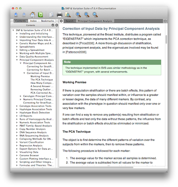What I really want to draw your attention to here is that even if you don't use SVS you can still view their manual online without registering, giving them your e-mail, or downloading any trialware. Think of this manual as an always up-to-date mega-review of GWAS - with it you can learn quite a bit about GWAS analysis, quality control, and statistics. For example, see this section on haplotype frequency estimation and the EM algorithm. The section on the mathematical motivation and implementation of the Eigenstrat PCA method explains the method perhaps better than the Eigenstrat paper and documentation itself. There are also lots of video tutorials that are helpful, even if you're not using SVS. This is a great resource, whether you're just trying to get a better grip on what PLINK is doing, or perhaps implementing some of these methods in your own software.

Support

Next, the support. After installing SVS on both my Mac laptop and the Linux box where I do my heavy lifting, one of the product specialists at Golden Helix called me and walked me through every step of a GWAS analysis, from QC to analysis to visualization. While analyzing the dbGaP data for my client I ran into both software-specific procedural issues as well as general scientific questions. If you've ever asked a basic question on the R-help mailing list, you know need some patience and a thick skin for all the RTFM responses you'll get. I was able to call the fine folks at Golden Helix and get both my technical and scientific questions answered in the same day. There are lots of resources for getting your questions answered, such as SEQanswers, Biostar, Cross Validated, and StackOverflow to name a few, but getting a forum response two days later from "SeqGeek96815" doesn't compare to having a team of scientists, statisticians, programmers, and product specialists on the other end of a telephone whose job it is to answer your questions.

Final Thoughts

This isn't meant to be a wholesale endorsement of Golden Helix or any other particular software company - I only wanted to share my experience stepping outside my comfortable open-source world into the walled garden of a commercially-licensed software from a for-profit company (the walls on the SVS garden aren't that high in reality - you can import and export data in any format imaginable). One of the nice things about command-line based tools is that it's relatively easy to automate a simple (or at least well-documented) process with tools like Galaxy, Taverna, or even by wrapping them with perl or bash scripts. However, the types of data my clients are collecting and the kinds of questions they're asking are always a little new and different, which means I'm rarely doing the same exact analysis twice. Because of the level of documentation and support provided to me, I was able to learn a new interface to a set of familiar procedures and run an analysis very quickly and without spending hours on forums figuring out why a particular program is seg-faulting. Will I abandon open-source tools like PLINK for SVS, Tophat-Cufflinks for CLC Workbench, BWA for NovoAlign, or R for Stata? Not in a million years. I haven't talked to Golden Helix or some of the above-mentioned companies about pricing for their products, but if I can spend a few bucks and save the time it would taken a full time technician at $50k+/year to write a new short read aligner or build a new SNP annotation database server, then I'll be able to provide a faster, high-quality, fiscally sustainable service at a much lower price for the core's clients, which is all-important in a time when federal funding is increasingly harder to come by.

Video Tip: Use Ensembl BioMart to Quickly Get Ortholog Information

A few weeks ago I showed you how to convert gene IDs with BioMart. Yesterday I hosted a workshop on the Ensembl Genome Browser, given by Dr. Bert Overduin from EBI-EMBL. He gave several examples of very useful tasks that you can do very quickly and easily using BioMart. One, in particular, is something that I'm doing for a client in the core right now.

Let's say you have a set of genes in one species and you want to know the orthologs in another species and gene expression probes in that species you can use to assay those orthologs. For example, Table 1 in this paper reports 25 gene expression probes that are dysregulated in humans when exposed to benzene. What if you only had the U133A/B Affymetrix probe IDs and wanted to know the gene names? What if you also wanted all the Ensembl gene IDs, names, and descriptions of the mouse orthologs for these human genes? Further, what are the mouse Affymetrix 430Av2 probe IDs that you can use to assay these genes' expression in mouse? All this can be accomplished for a list of genes in about 60 seconds using BioMart. See the video below. Watch it on Youtube in 1080p if you're having a hard time reading the text.



If you want to try this yourself, head to BioMart and copy the list of Affy probe IDs below:

207630_s_at
221840_at
219228_at
204924_at
227613_at
223454_at
228962_at
214696_at
210732_s_at
212371_at
225390_s_at
227645_at
226652_at
221641_s_at
202055_at
226743_at
228393_s_at
225120_at
218515_at
202224_at
200614_at
212014_x_at
223461_at
209835_x_at
213315_x_at

Youtube - Get Orthologs via BioMart

NSF BIGDATA webinar

If you're doing any kind of big data analysis - genomics, transcriptomics, proteomics, bioinformatics - then unless you've been on vacation the last few weeks you've no doubt heard about the NSF/NIH BIGDATA  Initiative (here's the NSF solicitation and here's the New York Times article about the funding opportunity). The solicitation "aims to advance core scientific and technological means of managing, analyzing, visualizing, and extracting useful information from large, diverse, distributed and heterogeneous data sets so as to: accelerate the progress of scientific discovery and innovation; lead to new fields of inquiry that would not otherwise be possible; encourage the development of new data analytic tools and algorithms; facilitate scalable, accessible, and sustainable data infrastructure; increase understanding of human and social processes and interactions; and promote economic growth and improved health and quality of life."

NSF is holding a webinar to describe the goals and focus of the BIGDATA solicitation, help investigators understand its scope, and answer any questions potential PIs might have.

The Webinar will be held from 11am-noon EST on May 8, 2012. Register here. The webinar will also be archived here a few days later.

NSF BIGDATA Webinar - May 8 2012

Awk Command to Count Total, Unique, and the Most Abundant Read in a FASTQ file

I was reading through a paper on comparative ChIP-Seq when I found this awk gem that lets you get some very basic stats very quickly on next generation sequencing reads. To use, simply cat the fastq file (or gunzip -c) and pipe that to this awk command:

cat myfile.fq | awk '((NR-2)%4==0){read=$1;total++;count[read]++}END{for(read in count){if(!max||count[read]>max) {max=count[read];maxRead=read};if(count[read]==1){unique++}};print total,unique,unique*100/total,maxRead,count[maxRead],count[maxRead]*100/total}'

The output would look something like this for some RNA-seq data downloaded from the Galaxy RNA-seq tutorial:

99115 60567 61.1078 ACCTCAGGA 354 0.357161

This is telling you:

1. The total number of reads (99,115).
2. The number of unique reads (60,567).
3. The frequency of unique reads as a proportion of the total (61%).
4. The most abundant sequence (useful for finding adapters, linkers, etc).
5. The number of times that sequence is present (354).
6. The frequency of that sequence as a proportion of the total number of reads (0.35%).

If you have a handful of fastq files in a directory and you'd like to do this for each of them, you can wrap this in a for loop in bash:

for read in `ls *.fq`; do echo -n "$read "; awk '((NR-2)%4==0){read=$1;total++;count[read]++}END{for(read in count){if(!max||count[read]>max) {max=count[read];maxRead=read};if(count[read]==1){unique++}};print total,unique,unique*100/total,maxRead,count[maxRead],count[maxRead]*100/total}' $read; done

This does the same thing, but adds an extra field at the beginning for the file name. I haven't yet figured out how to wrap this into GNU parallel, but the for loop should do the trick for multiple files.

Check out FASTQC for more extensive quality assessment.

RNA-Seq Methods & March Twitter Roundup

There were lots of interesting developments this month that didn't work their way into a full blog post. Here is an incomplete list of what I've been tweeting about over the last few weeks. But first I want to draw your attention to the latest manuscript for a new bioconductor package for doing RNA-seq in R.

DEXSeq vs Cuffdiff. See the pre-publication manuscript from Simon Anders, Alejandro Reyes, and Wolfgang Huber: "Detecting differential usage of exons from RNA-Seq data." DEXSeq is an R package by the same guys who developed the DESeq R package and the HTSeq python scripts. (Incidentally, both DESeq and DEXSeq are rare examples of bioconductor vignettes which are well developed and are a pleasure to read). I often use cufflinks/cuffdiff in the bioinformatics core was because many other tools and methods only allow you to interrogate differential expression at the gene level. Using cufflinks for transcriptome assembly enables you to interrogate transcript/isoform expression, differential splicing, differential coding output, differential promoter usage, etc. DEXSeq uses similar methodology as DESeq, but can give you exon-level differential expression, without going through all the assembly business that cufflinks does. In one of the supplementary tables in their pre-pub manuscript, they compare several versions of cuffdiff to DEXSeq on two datasets. Both of these datasets had biological replicates for treatment and control conditions. They compared treatment to controls, and found DEXseq gave you more significant hits than cuffdiff. Then they compared controls to other controls (ideally should have zero hits) and found cufflinks had way more hits. See p13, p23, tables S1 and S2.

Proper comparison treatment vs control, # significant hits:

DEXSeq: 159

Cuffdiff 1.1: 145

Cuffdiff 1.2: 69

Cuffdiff 1.3: 50

Mock comparison controls vs controls, # significant hits:

DEXSeq: 8

Cuffdiff 1.1: 314

Cuffdiff 1.2: 650

Cuffdiff 1.3: 639

In the UVA Bioinformatics core we strive for reproducibility, scalability, and transparency using the most robust tools and methodology available. It gives me pause to see such alarmingly different results with each new version and each new protocol of a particular tool. What are your thoughts and experiences with using Cufflinks/Cuffdiff, DESeq/DEXSeq, or the many, many other tools for RNA-Seq (MISO, ExpressionPlot, EdgeR, RSEM, easyRNASeq, etc.)? Please share in the comments.

Everything else:

Webinar from @goldenhelixinc: Learning From Our GWAS Mistakes: From experimental design to scientific method https://t.co/KkxAn18p

Sequencing technology does not eliminate biological variability http://t.co/NI3acZgn

[bump] Questions on cutoff setting of FPKM value & know genes filtering in Cuffmerge result http://t.co/iKMZ7Dsd #bioinformatics

Very cool: DNAse-Seq+RNA-seq used to show DNaseI sensitivity eQTLs are a major determinant of gene expression variation http://t.co/nPo3xHVa

Beware using UCSC GTFs in HTSeq/CovergeBed for counting RNA-seq reads. "transcript_id" is repeated as "gene_id"! https://t.co/ADg1Pi6U

Google Scholar Metrics: top 20 journals in bioinformatics http://t.co/QYTf5pyT

A systematic eQTL study of cis-trans #epistasis in 210 HapMap individuals http://t.co/0YHlFQak

Identification of allele-specific alternative mRNA processing via RNA-seq http://t.co/fig9cLlH #bioinformatics @myen

prepub on arXiv + analysis tutorial/walkthrough + AWS EC2 AMI + git repo + ipython notebook = reproducible research done right http://t.co/GPNmpdJD

Altmetrics in the Wild: Using Social Media to Explore Scholarly Impact http://t.co/8xZuIHw9

NSF-NIH Interagency Initiative: Core Techniques and Technologies for Advancing Big Data Science and Engineering http://t.co/W3LUdCsG

New approach from @MarylynRitchie lab to collapsing/combining: using biological pathways rather than positional info http://t.co/ywWj0MNn

The Transcription Factor Encyclopedia http://t.co/DjJUwR10 Paper: http://t.co/b0J8PXO6

NF-kB: where did it come from and why? http://t.co/NLV1mBd0

Cloud BioLinux: pre-configured and on-demand #bioinformatics computing for the genomics community. @myen http://t.co/3kCE0ktH

SCOTUS remands AMP v Myriad (BRCA) patent case to CAFC to consider in light of prometheus decision http://t.co/7CkTa4l0

57 year experiment, Drosophila kept in dark for 1400 generations, many evolutionary changes (record longest postdoc!) http://t.co/wukq8fAf

IsoLasso: a LASSO regression approach to RNA-Seq based transcriptome assembly http://t.co/FN1sYM8f #bioinformatics

Complex disease genetics is complex. Imagine that. Hirschhorn, Visscher, & the usual consortium suspects: http://t.co/Bwopxlx6

MAnorm: a robust model for quantitative comparison of ChIP-Seq data sets http://t.co/pffuHIlO #bioinformatics

Paper about SEQanswers forum published in #Bioinformatics http://t.co/SUlQ6O8c

num-utils - like awk, grep, sort, cut, etc for numbers http://t.co/bgkB5FMV

Nat Protocols: Differential gene & transcript expression analysis of RNA-seq w/ TopHat & Cufflinks http://t.co/U1ZpSE7V #bioinformatics