Microbiome Digest Blog

I have a noteworthy blogs tag on this blog that I sort of forgot about, and haven't used in years. But I started reading one recently that's definitely qualified for the distinction.

The Microbiome Digest is written by Elisabeth Bik, a scientist studying the microbiome at Stanford. It's a near-daily compilation of papers and popular press articles mostly relating to microbiome research, split up into categories like the human microbiome, the non-human microbiome (soil, animal, plants, other environments), metagenomics and bioinformatics methods, reviews, news articles, and other general science or career advice articles.

I imagine Elisabeth spends hours each week culling the huge onslaught of literature into these highly relevant digests. I wish someone else would do the same for other areas I care about so I don't have to. I subscribe to the RSS feed and the email list so I never miss a post. If you're at all interested in metagenomics or microbiome research, I suggest you do the same!

Microbiome Digest

Using the microbenchmark package to compare the execution time of R expressions

I recently learned about the microbenchmark package while browsing through Hadley’s advanced R programming book. I’ve done some quick benchmarking using system.time() in a for loop and taking the average, but the microbenchmark function in the microbenchmark package makes this much easier. Hadley gives the example of taking the square root of a vector using the built-in sqrt function versus the mathematical equivalent of raising the vector to the power of 0.5.

library(microbenchmark)
x = runif(100)
microbenchmark(
  sqrt(x),
  x ^ 0.5
)

By default, microbenchmark runs each argument 100 times to get an average look at how long each evaluation takes. Results:

Unit: nanoseconds
    expr  min     lq    mean median     uq   max neval
 sqrt(x)  825  860.5 1212.79  892.5  938.5 12905   100
   x^0.5 3015 3059.5 3776.81 3101.5 3208.0 15215   100

On average sqrt(x) takes 1212 nanoseconds, compared to 3776 for x^0.5. That is, the built-in sqrt function is about 3 times faster. (This was surprising to me. Anyone care to comment on why this is the case?)

Now, let’s try it on something just a little bigger. This is similar to a real-life application I faced where I wanted to compute summary statistics of some value grouping by levels of some other factor. In the example below we’ll use the nycflights13 package, which is a data package that has info on 336,776 outbound flights from NYC in 2013. I’m going to go ahead and load the dplyr package so things print nicely.

library(dplyr)
library(nycflights13)
flights

Source: local data frame [336,776 x 16]

year month day dep_time dep_delay arr_time arr_delay carrier tailnum
1  2013     1   1      517         2      830        11      UA  N14228
2  2013     1   1      533         4      850        20      UA  N24211
3  2013     1   1      542         2      923        33      AA  N619AA
4  2013     1   1      544        -1     1004       -18      B6  N804JB
5  2013     1   1      554        -6      812       -25      DL  N668DN
6  2013     1   1      554        -4      740        12      UA  N39463
7  2013     1   1      555        -5      913        19      B6  N516JB
8  2013     1   1      557        -3      709       -14      EV  N829AS
9  2013     1   1      557        -3      838        -8      B6  N593JB
10 2013     1   1      558        -2      753         8      AA  N3ALAA
..  ...   ... ...      ...       ...      ...       ...     ...     ...
Variables not shown: flight (int), origin (chr), dest (chr), air_time
(dbl), distance (dbl), hour (dbl), minute (dbl)

Let’s say we want to know the average arrival delay (arr_delay) broken down by each airline (carrier). There’s more than one way to do this.

Years ago I would have used the built-in aggregate function.

aggregate(flights$arr_delay, by=list(flights$carrier), mean, na.rm=TRUE)

This gives me the results I’m looking for:

   Group.1          x
1       9E  7.3796692
2       AA  0.3642909
3       AS -9.9308886
4       B6  9.4579733
5       DL  1.6443409
6       EV 15.7964311
7       F9 21.9207048
8       FL 20.1159055
9       HA -6.9152047
10      MQ 10.7747334
11      OO 11.9310345
12      UA  3.5580111
13      US  2.1295951
14      VX  1.7644644
15      WN  9.6491199
16      YV 15.5569853

Alternatively, you can use the sqldf package, which feels natural if you’re used to writing SQL queries.

library(sqldf)
sqldf("SELECT carrier, avg(arr_delay) FROM flights GROUP BY carrier")

Not long ago I learned about the data.table package, which is good at doing these kinds of operations extremely fast.

library(data.table)
flightsDT = data.table(flights)
flightsDT[ , mean(arr_delay, na.rm=TRUE), carrier]

Finally, there’s my new favorite, the dplyr package, which I covered recently.

library(dplyr)
flights %>% group_by(carrier) %>% summarize(mean(arr_delay, na.rm=TRUE))

Each of these will give you the same result, but which one is faster? That’s where the microbenchmark package becomes handy. Here, I’m passing all four evaluations to the microbenchmark function, and I’m naming those “base”, “sqldf”, “datatable”, and “dplyr” so the output is easier to read.

library(microbenchmark)
mbm = microbenchmark(
  base = aggregate(flights$arr_delay, by=list(flights$carrier), mean, na.rm=TRUE),
  sqldf = sqldf("SELECT carrier, avg(arr_delay) FROM flights GROUP BY carrier"),
  datatable = flightsDT[ , mean(arr_delay, na.rm=TRUE), carrier],
  dplyr = flights %>% group_by(carrier) %>% summarize(mean(arr_delay, na.rm=TRUE)),
  times=50
)
mbm

Here’s the output:

Unit: milliseconds
      expr     min      lq    mean  median      uq     max neval
      base 1487.39 1521.12 1544.73 1539.96 1554.55 1676.25    50
     sqldf  867.14  880.34  892.24  887.88  897.28  982.91    50
 datatable    4.12    4.57    5.29    4.89    5.43   18.69    50
     dplyr   14.49   15.53   16.59   15.86   16.58   25.04    50

In this example, data.table was clearly the fastest on average. dplyr took ~3 times longer, sqldf took ~180x longer, and the base aggregate function took over 300 times longer. Let’s visualize those results using ggplot2 (microbenchmark has an autoplot method available, and note the log scale):

library(ggplot2)
autoplot(mbm)

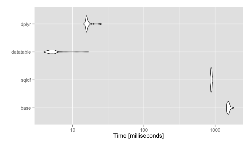
In this example data.table and dplyr were both relatively fast, with data.table being just a few milliseconds faster. Sometimes this will matter, other times it won’t. This is a matter of personal preference, but I personally find the data.table incantation not the least bit intuitive compared to dplyr. The way we pronounce flights %>% group_by(carrier) %>% summarize(mean(arr_delay, na.rm=TRUE)) is: “take flights then group that data by the carrier variable then summarize the data taking the mean of arr_delay.” The dplyr syntax, for me, is much easier to use and extend to much more complex data management and analysis tasks, so I’ll sacrifice those few milliseconds or program run time for the minutes or hours of programmer debugging time. But if you’re planning on running a piece of code on, for instance, millions or more simulations, then those few milliseconds might be important to you. The microbenchmark package makes benchmarking easy for small pieces of code like this.

The code used for this analysis is consolidated here on GitHub

​

Importing Illumina BeadArray data into R

A colleague needed some help getting Illumina BeadArray gene expression data loaded into R for data analysis with limma. Hopefully whoever ran your arrays can export the data as text files formatted as described in the code below. If so, you can import those text files directly using the beadarray package. This way you avoid getting bogged down with GenomeStudio, which requires a license (ugh) and only runs on Windows (ughhh). Here's how I do it.

RNA-seq Data Analysis Course Materials

Last week I ran a one-day workshop on RNA-seq data analysis in the UVA Health Sciences Library. I set up an AWS public EC2 image with all the necessary software installed. Participants logged into AWS, launched the image, and we kicked off the morning session with an introduction to the Unix shell (taught by Jessica Bonnie, a biostatistician here in our genomics group, and a fellow Software Carpentry instructor). I followed with a walkthrough of using FastQC for quality assessment, FASTX toolkit for trimming, TopHat for alignment, and featureCounts to summarize gene expression read counts at the gene level. I started the afternoon session started with an introduction to R, followed by a tutorial on analyzing the count data we generated in the first part using DESeq2 in R.

All of the rendered course material is available here. The source code used to generate this material is all on available on GitHub (go read my post on collaborative lesson development, if you haven't already). Much of the introductory Unix lesson material was adapted from the Software Carpentry and Data Carpentry projects.

I wrote a more thorough blog post about how the course went here on the Software Carpentry blog.

I also compiled a PDF of all the course materials, available on Figshare: http://dx.doi.org/10.6084/m9.figshare.1247658.

Operate on the body of a file but not the header

Sometimes you need to run some UNIX command on a file but only want to operate on the body of the file, not the header. Create a file called body somewhere in your $PATH, make it executable, and add this to it:

#!/bin/bash
IFS= read -r header
printf '%s\n' "$header"
eval $@

Now, when you need to run something but ignore the header, use the body command first. For example, we can create a simple data set with a header row and some numbers:

$ echo -e "header\n1\n5\n4\n7\n3"
header
1
5
4
7
3

We can pipe the whole thing to sort:

$ echo -e "header\n1\n5\n4\n7\n3" | sort
1
3
4
5
7
header

Oops, we don’t want the header to be included in the sort. Let’s use the body command to operate only on the body, skipping the header:

$ echo -e "header\n1\n5\n4\n7\n3" | body sort
header
1
3
4
5
7

Sure, there are other ways to solve the problem with sort, but body will solve many more problems. If you have multiple header rows, just call body multiple times.

Inspired by this post on Stack Exchange.

​

R package to convert statistical analysis objects to tidy data frames

I talked a little bit about tidy data my recent post about dplyr, but you should really go check out Hadley’s paper on the subject.

R expects inputs to data analysis procedures to be in a tidy format, but the model output objects that you get back aren’t always tidy. The reshape2, tidyr, and dplyr are meant to take data frames, munge them around, and return a data frame. David Robinson's broom package bridges this gap by taking un-tidy output from model objects, which are not data frames, and returning them in a tidy data frame format.

(From the documentation): if you performed a linear model on the built-in mtcars dataset and view the object directly, this is what you’d see:

lmfit = lm(mpg ~ wt, mtcars)
lmfit

Call:
lm(formula = mpg ~ wt, data = mtcars)

Coefficients:
(Intercept)           wt  
     37.285       -5.344

summary(lmfit)

Call:
lm(formula = mpg ~ wt, data = mtcars)

Residuals:
   Min     1Q Median     3Q    Max 
-4.543 -2.365 -0.125  1.410  6.873 

Coefficients:
            Estimate Std. Error t value Pr(>|t|)    
(Intercept)   37.285      1.878   19.86  < 2e-16 ***
wt            -5.344      0.559   -9.56  1.3e-10 ***
---
Signif. codes:  0 '***' 0.001 '**' 0.01 '*' 0.05 '.' 0.1 ' ' 1

Residual standard error: 3.05 on 30 degrees of freedom
Multiple R-squared:  0.753,  Adjusted R-squared:  0.745 
F-statistic: 91.4 on 1 and 30 DF,  p-value: 1.29e-10

If you’re just trying to read it this is good enough, but if you’re doing other follow-up analysis or visualization, you end up hacking around with str() and pulling out coefficients using indices, and everything gets ugly quick.

But the tidy function in the broom package run on the fit object probably gives you what you were looking for in a tidy data frame:

tidy(lmfit)

         term estimate stderror statistic   p.value
1 (Intercept)   37.285   1.8776    19.858 8.242e-19
2          wt   -5.344   0.5591    -9.559 1.294e-10

The tidy() function also works on other types of model objects, like those produced by glm() and nls(), as well as popular built-in hypothesis testing tools like t.test(), cor.test(), or wilcox.test().

View the README on the GitHub page, or install the package and run the vignette to see more examples and conventions.

broom: Convert statistical analysis objects from R into tidy format

​

UVA / Charlottesville R Meetup

TL;DR? We started an R Users group, awesome community, huge turnout at first meeting, lots of potential.

---

I've sat through many hours of meetings where faculty lament the fact that their trainees (and the faculty themselves!) are woefully ill-prepared for our brave new world of computing- and data-intensive science. We've started to address this by running annual Software Carpentry bootcamps (March 2013, and March 2014). To make things more sustainable, we're running our own Software Carpentry instructor training here later this month, where we'll train scientists how to teach other scientists basic computing skills like using UNIX, programming in Python or R, version control, automation, and testing. I went through this training course online a few months ago, and it was an excellent introduction to pedagogy and the psychology of learning (let's face it, most research professors were never taught how to teach; it's a skill you learn, not one you inherit with the initials behind your name).

Something that constantly comes up in these conversations is how to promote continued learning and practice after the short bootcamp is over. Students get a whirlwind tour of scientific computing skills over two days, but there's generally very little follow-up that's necessary to encourage continued practice and learning.

At the same time we've got a wide variety of scientists spanning all disciplines including social sciences, humanities, medicine, physics, chemistry, math, and engineering that are doing scientific computing and data analysis on a daily basis who could really benefit from learning from one another.

These things motivated us to start a local R Users Group. So far we have 118 people registered on Meetup.com, and this week we had an excellent turnout at our first meeting, with over 70 people who RSVP'd.

At this first meetup we kicked things off with an introduction to the group, why we started it, and our goals. I then launched into a quick demo of some of the finer features in the dplyr package for effortless advanced data manipulation and analysis. The meetup group has a GitHub repository where all the code from our meetups will be stored. Finally, we concluded with a discussion of topics the group would like to see presented in the future: ggplot2, R package creation, reproducible research, dynamic documentation, and web scraping were a few of the things mentioned. We collectively decided that either talks could be either research talks highlighting how these things were used in an actual research project, or they could be demo/tutorial in nature, like the dplyr talk I gave.

The rich discussion we had at the end of this session really highlighted the potential this community has. In addition to the diversity and relative gender-balance we saw in our first meetup's participants, we had participants from all over UVA as well as representation from local industry and non-profit organizations.

I, for one, am tremendously excited about this new community, and will post the occasional update from the group here on this blog.

GNU datamash

GNU datamash is a command-line utility that offers simple calculations (e.g. count, sum, min, max, mean, stdev, string coalescing) as well as a rich set of statistical functions, to quickly assess information in textual input files or from a UNIX pipe. Here are a few examples:

E.g., let’s use the seq command to generate some data, and use datamash sum to add up all the values in the first column:

$ seq 5
1
2
3
4
5
$ seq 5 | datamash sum 1
15

What else? Let’s calculate the mean, 1st quartile, median, 3rd quarile, IQR, sample-standard-deviation, and p-value of Jarque-Bera test for normal distribution, using some data in file.txt:

$ cat file.txt | datamash -H mean 1 q1 1 median 1 q3 1 iqr 1 sstdev 1 jarque 1
mean(x)   q1(x)  median(x)  q3(x)   iqr(x)  sstdev(x)  jarque(x)
45.32     23     37         61.5    38.5    30.4487    8.0113e-09

Go take a look at more examples, specifically the examples using datamash to parse a GTF file. Datamash can very quickly do things like find the number of isoforms per gene by grouping (collapsing) over gene IDs and counting the number of transcripts, find the number of genes with more than 5 isoforms, find genes transcribed from multiple chromosomes, examine variability in exon counts per gene, etc.

GNU datamash

​