Using the microbenchmark package to compare the execution time of R expressions

I recently learned about the microbenchmark package while browsing through Hadley’s advanced R programming book. I’ve done some quick benchmarking using system.time() in a for loop and taking the average, but the microbenchmark function in the microbenchmark package makes this much easier. Hadley gives the example of taking the square root of a vector using the built-in sqrt function versus the mathematical equivalent of raising the vector to the power of 0.5.

library(microbenchmark)
x = runif(100)
microbenchmark(
  sqrt(x),
  x ^ 0.5
)

By default, microbenchmark runs each argument 100 times to get an average look at how long each evaluation takes. Results:

Unit: nanoseconds
    expr  min     lq    mean median     uq   max neval
 sqrt(x)  825  860.5 1212.79  892.5  938.5 12905   100
   x^0.5 3015 3059.5 3776.81 3101.5 3208.0 15215   100

On average sqrt(x) takes 1212 nanoseconds, compared to 3776 for x^0.5. That is, the built-in sqrt function is about 3 times faster. (This was surprising to me. Anyone care to comment on why this is the case?)

Now, let’s try it on something just a little bigger. This is similar to a real-life application I faced where I wanted to compute summary statistics of some value grouping by levels of some other factor. In the example below we’ll use the nycflights13 package, which is a data package that has info on 336,776 outbound flights from NYC in 2013. I’m going to go ahead and load the dplyr package so things print nicely.

library(dplyr)
library(nycflights13)
flights

Source: local data frame [336,776 x 16]

year month day dep_time dep_delay arr_time arr_delay carrier tailnum
1  2013     1   1      517         2      830        11      UA  N14228
2  2013     1   1      533         4      850        20      UA  N24211
3  2013     1   1      542         2      923        33      AA  N619AA
4  2013     1   1      544        -1     1004       -18      B6  N804JB
5  2013     1   1      554        -6      812       -25      DL  N668DN
6  2013     1   1      554        -4      740        12      UA  N39463
7  2013     1   1      555        -5      913        19      B6  N516JB
8  2013     1   1      557        -3      709       -14      EV  N829AS
9  2013     1   1      557        -3      838        -8      B6  N593JB
10 2013     1   1      558        -2      753         8      AA  N3ALAA
..  ...   ... ...      ...       ...      ...       ...     ...     ...
Variables not shown: flight (int), origin (chr), dest (chr), air_time
(dbl), distance (dbl), hour (dbl), minute (dbl)

Let’s say we want to know the average arrival delay (arr_delay) broken down by each airline (carrier). There’s more than one way to do this.

Years ago I would have used the built-in aggregate function.

aggregate(flights$arr_delay, by=list(flights$carrier), mean, na.rm=TRUE)

This gives me the results I’m looking for:

   Group.1          x
1       9E  7.3796692
2       AA  0.3642909
3       AS -9.9308886
4       B6  9.4579733
5       DL  1.6443409
6       EV 15.7964311
7       F9 21.9207048
8       FL 20.1159055
9       HA -6.9152047
10      MQ 10.7747334
11      OO 11.9310345
12      UA  3.5580111
13      US  2.1295951
14      VX  1.7644644
15      WN  9.6491199
16      YV 15.5569853

Alternatively, you can use the sqldf package, which feels natural if you’re used to writing SQL queries.

library(sqldf)
sqldf("SELECT carrier, avg(arr_delay) FROM flights GROUP BY carrier")

Not long ago I learned about the data.table package, which is good at doing these kinds of operations extremely fast.

library(data.table)
flightsDT = data.table(flights)
flightsDT[ , mean(arr_delay, na.rm=TRUE), carrier]

Finally, there’s my new favorite, the dplyr package, which I covered recently.

library(dplyr)
flights %>% group_by(carrier) %>% summarize(mean(arr_delay, na.rm=TRUE))

Each of these will give you the same result, but which one is faster? That’s where the microbenchmark package becomes handy. Here, I’m passing all four evaluations to the microbenchmark function, and I’m naming those “base”, “sqldf”, “datatable”, and “dplyr” so the output is easier to read.

library(microbenchmark)
mbm = microbenchmark(
  base = aggregate(flights$arr_delay, by=list(flights$carrier), mean, na.rm=TRUE),
  sqldf = sqldf("SELECT carrier, avg(arr_delay) FROM flights GROUP BY carrier"),
  datatable = flightsDT[ , mean(arr_delay, na.rm=TRUE), carrier],
  dplyr = flights %>% group_by(carrier) %>% summarize(mean(arr_delay, na.rm=TRUE)),
  times=50
)
mbm

Here’s the output:

Unit: milliseconds
      expr     min      lq    mean  median      uq     max neval
      base 1487.39 1521.12 1544.73 1539.96 1554.55 1676.25    50
     sqldf  867.14  880.34  892.24  887.88  897.28  982.91    50
 datatable    4.12    4.57    5.29    4.89    5.43   18.69    50
     dplyr   14.49   15.53   16.59   15.86   16.58   25.04    50

In this example, data.table was clearly the fastest on average. dplyr took ~3 times longer, sqldf took ~180x longer, and the base aggregate function took over 300 times longer. Let’s visualize those results using ggplot2 (microbenchmark has an autoplot method available, and note the log scale):

library(ggplot2)
autoplot(mbm)

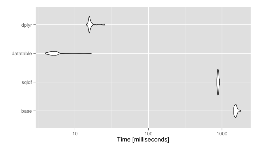
In this example data.table and dplyr were both relatively fast, with data.table being just a few milliseconds faster. Sometimes this will matter, other times it won’t. This is a matter of personal preference, but I personally find the data.table incantation not the least bit intuitive compared to dplyr. The way we pronounce flights %>% group_by(carrier) %>% summarize(mean(arr_delay, na.rm=TRUE)) is: “take flights then group that data by the carrier variable then summarize the data taking the mean of arr_delay.” The dplyr syntax, for me, is much easier to use and extend to much more complex data management and analysis tasks, so I’ll sacrifice those few milliseconds or program run time for the minutes or hours of programmer debugging time. But if you’re planning on running a piece of code on, for instance, millions or more simulations, then those few milliseconds might be important to you. The microbenchmark package makes benchmarking easy for small pieces of code like this.

The code used for this analysis is consolidated here on GitHub

​