Use nanoparquet instead of readr/CSV

 This is reposted from the original at https://blog.stephenturner.us/p/use-nanoparquet-instead-of-readr-csv.

Parquet is interoperable between Python and R, fast to read+write, works well with databases, and stores complex data types (e.g., tibble listcols). Use it instead of CSV. Many pros, few (no?) cons.

Yesterday I wrote about base R vs. dplyr vs. duckdb for a simple summary analysis. In that post I simulated 100 million rows of a dataset and wrote to disk as CSV. I then benchmarked how long it took to read in and compute a simple grouped mean.

DuckDB vs dplyr vs base R

Stephen Turner

·

Oct 7

Read full story

One thing I didn’t do here was separate the time it took to read data into memory (for base R and dplyr) versus computing the actual summary. Remember, with DuckDB you don’t actually have to read the data into memory for SQL operations you can do with DuckDB or duckplyr.

After I wrote this I downloaded the materials from Hadley Wickham’s R in Production workshop from posit::conf(2024) where he encourages using parquet instead of CSV for saving and sharing data.

Why parquet? From the slides:

• Like csv, every language can read and write.

• Binary column-oriented format (much faster to read).

• Rich type system (including missing values).

• Efficient encodings + optional compression (smaller files).

• Data stored in "chunks" (can work in parallel & don't need to read entire file).

• Supports complex data types (e.g. list-columns).

• Many modern databases can use parquet files directly.

In these slides I also learned about the nanoparquet package — a zero dependency package for reading and writing parquet files in R. Besides all the benefits noted above, parquet is much faster to read and write. And, as opposed to saving as .rds, parquet can easily be passed back and forth between R, Python, and other frameworks.

Let’s take a look at how reading and writing parquet files compares with CSV, either with base R or readr.

Read/write speed with base R, readr, nanoparquet

First, load the libraries I’ll use here.

library(tidyverse)
library(nanoparquet)

Next, simulate 100 million rows, 5 columns of numeric, categorical, and date data.

n <- 1e8
set.seed(42)
dat <-
  tibble(
    id = sample(n/10, n, replace = TRUE),
    category = sample(letters, n, replace = TRUE),
    value1 = rnorm(n),
    value2 = runif(n, min = 0, max = 1000),
    date = sample(seq.Date(from = as.Date("2010-01-01"),
                           to = as.Date("2020-12-31"),
                           by = "day"),
                  size=n,
                  replace = TRUE)) |>
  arrange(id, category, date)

The data looks like this:

# A tibble: 100,000,000 × 5
      id category value1 value2 date
   <int> <chr>     <dbl>  <dbl> <date>
 1     1 b        -1.26   145.  2020-02-15
 2     1 g        -0.316  157.  2020-06-03
 3     1 i        -1.42   919.  2019-11-24
 4     1 k         0.592  349.  2011-06-15
 5     1 l        -0.292  650.  2013-03-19
 6     1 m         0.316  802.  2015-05-25
 7     1 q         0.112  470.  2020-07-13
 8     1 t         0.637  236.  2011-02-26
 9     1 w         1.72    49.5 2016-02-25
10     2 a        -0.572  506.  2018-01-22
# ℹ 99,999,990 more rows

Next, I’ll create a list holding the time it takes to read and write using base R, readr, and nanoparquet. Notice that readr will attempt to guess the column types when reading in data, by default using only the first 1,000 rows. This could lead to problems if your first 1,000 rows contained numeric values, but later on in the file you have strings or other data types.

time <- list()
time$write.csv <- system.time(write.csv(dat, "dat.csv"))
time$write_csv <- system.time(write_csv(dat, "dat.csv"))
time$write_pqt <- system.time(write_parquet(dat, "dat.parquet"))
time$read.csv  <- system.time(read.csv("dat.csv"))
time$read_csv  <- system.time(read_csv("dat.csv"))
time$read_pqt  <- system.time(read_parquet("dat.parquet"))

Finally, extract the timing into a data frame, then plot.

time |>
  map_dbl("elapsed") |>
  enframe("fn", "seconds") |>
  mutate(task=ifelse(grepl("write", fn), "write", "read")) |>
  mutate(pkg=case_when(
    grepl("\\.csv$", fn) ~ "base_R",
    grepl("_csv$", fn) ~ "readr",
    grepl("_pqt$", fn) ~ "nanoparquet"
  )) |>
  mutate(pkg=fct_relevel(pkg, "base_R", "readr", "nanoparquet")) |>
  ggplot(aes(task, seconds, fill=pkg)) +
  geom_col(position="dodge") +
  theme_classic() +
  labs(x="Task", y="Time (seconds)", fill=NULL) + 
  theme(legend.position="bottom")

The results are compelling:

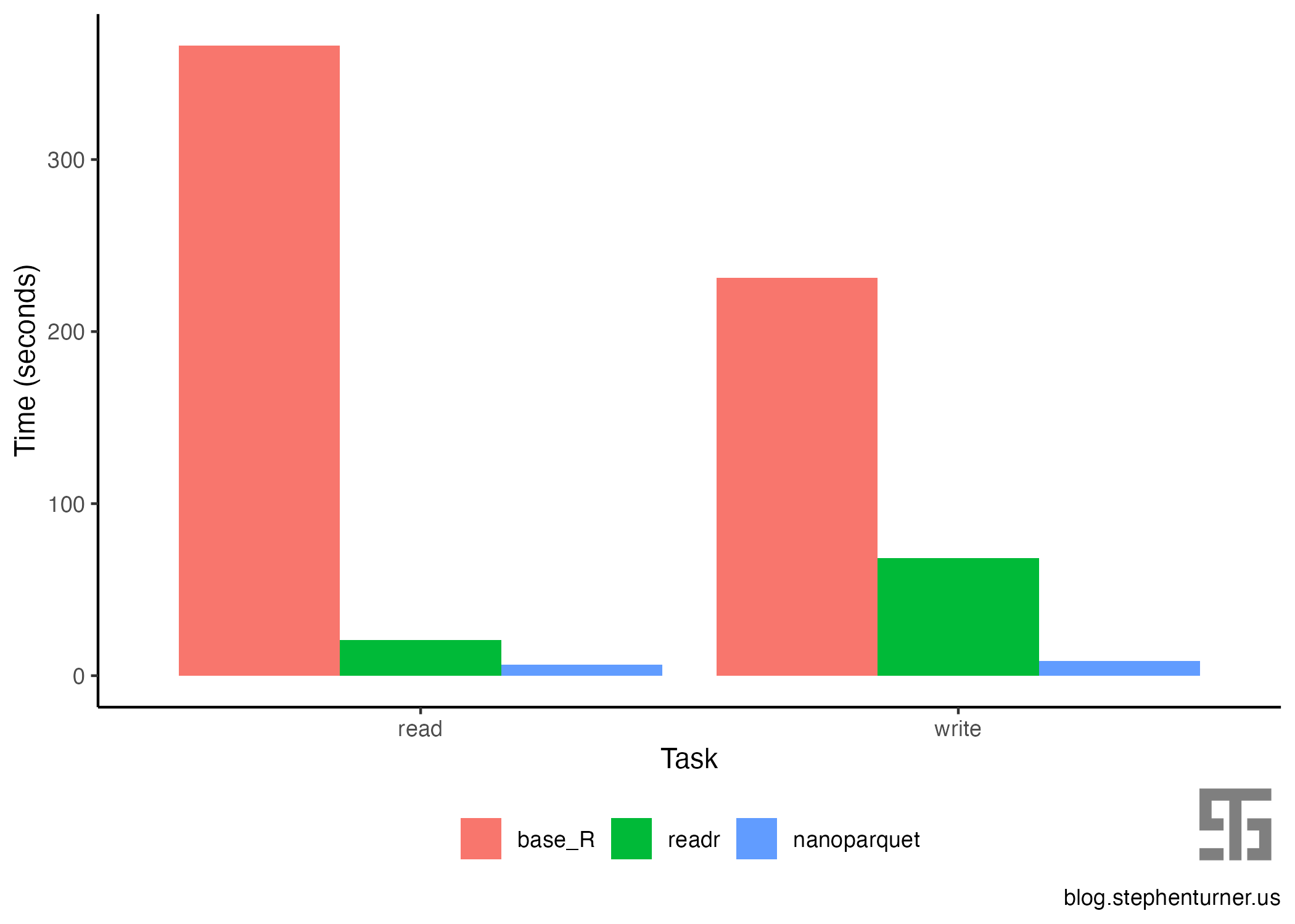
In tabular form:

task   base_R  readr  nanoparquet
read      366     21            6
write     231     68            8

Writing with nanoparquet is 29x faster than base R, and 8.5x faster than readr. Reading with nanoparquet is 61x faster than base R, 3.5x faster than readr. With the added bonus of column types coming in as the types they were originally created as (id as integer, the date column as an actual date). Additionally, the CSV is 5.5 Gb on disk (which could be compressed), and the parquet file is only 1.9 Gb.

Inspecting parquet files

As noted above, another nice feature of using parquet is the ability to store column types as they were originally created, rather than relying on readr::read_csv() to correctly guess the column type (or supply column types explicitly).

The nanoparquet package has a few other functions that allow us to see various kinds of metadata about the parquet files on disk without actually reading them in. From the documentation:

• parquet_info() shows a basic summary of the file.

• parquet_column_types() shows the leaf columns, these are are the ones that read_parquet() reads into R.

• parquet_schema() shows all columns, including non-leaf columns.

• parquet_metadata() shows the most complete metadata information: file meta data, the schema, the row groups and column chunks of the file.

> parquet_info("dat.parquet")
# A data frame: 1 × 7
  file_name   num_cols  num_rows ...
  <chr>          <int>     <dbl> ...
1 dat.parquet        5 100000000 ...

> parquet_column_types("dat.parquet")
# A data frame: 5 × 5
  file_name   name     type       r_type    logical_type
* <chr>       <chr>    <chr>      <chr>     <I<list>>
1 dat.parquet id       INT32      integer   <INT(32, TRUE)>
2 dat.parquet category BYTE_ARRAY character <STRING>
3 dat.parquet value1   DOUBLE     double    <NULL>
4 dat.parquet value2   DOUBLE     double    <NULL>
5 dat.parquet date     INT32      Date      <DATE>

Direct analysis on parquet with DuckDB+duckplyr

Similar to what was demonstrated in the previous post, we can run a query on this data to summarize values grouped by ID for all ~10 million groups in this data using duckplyr as an interface to DuckDB, without ever having to actually read the parquet files into memory. Here’s how to do that (the nrow() at the end actually materializes the resulting data frame into a tibble in your R session).

Similar to the previous post, this summary analysis took about 3.2 seconds on 100 million rows, without actually having to read the data into memory.

library(duckplyr)
system.time({
  res <- 
    duckplyr_df_from_parquet("dat.parquet") |>
    summarize(
      mean_value1 = mean(value1),
      mean_value2 = mean(value2),
      .by=id) |>
    arrange(id)
  nrow(res)
})

Results preview:

# A tibble: 9,999,521 × 3
      id mean_value1 mean_value2
   <int>       <dbl>       <dbl>
 1     1     0.00983        420.
 2     2    -0.379          661.
 3     3    -0.0515         491.
 4     4     0.0574         542.
 5     5    -0.173          398.
 6     6     0.0854         405.
 7     7     0.200          510.
 8     8     0.0117         621.
 9     9    -0.0726         470.
10    10    -0.456          503.
# ℹ 9,999,511 more rows

If you’d rather write raw SQL instead of using duckplyr, you can do that too. This also takes 3.2 seconds for 100 million rows.

library(DBI)
library(duckdb)
system.time({
  conn <- dbConnect(duckdb())
  res <-
    dbGetQuery(conn = conn,
               statement="
                     SELECT id,
                     AVG(value1) as mean_value1,
                     AVG(value2) as mean_value2
                     FROM read_parquet('dat.parquet')
                     GROUP BY id
                     ORDER BY id")
  dbDisconnect(conn, shutdown=TRUE)
})