PLATO, an Alternative to PLINK

Since the near beginning of genome-wide association studies, the PLINK software package (developed by Shaun Purcell’s group at the Broad Institute and MGH) has been the standard for manipulating the large-scale data produced by these studies.  Over the course of its development, numerous features and options were added to enhance its capabilities, but it is best known for the core functionality of performing quality control and standard association tests. 

Nearly 10 years ago (around the time PLINK was just getting started), the CHGR Computational Genomics Core (CGC) at Vanderbilt University started work on a similar framework for implementing genotype QC and association tests.  This project, called PLATO, has stayed active primarily to provide functionality and control that (for one reason or another) is unavailable in PLINK.  We have found it especially useful for processing ADME and DMET panel data – it supports QC and association tests of multi-allelic variants.    

PLATO runs via command line interface, but accepts a batch file that allows users to specify an order of operations for QC filtering steps.  When running multiple QC steps in a single run of PLINK, the order of application is hard-coded and not well documented.  As a result, users wanting this level of control must run a sequence of PLINK commands, generating new data files at each step leading to longer compute times and disk usage.  PLATO also has a variety of data reformatting options for other genetic analysis programs, making it easy to run EIGENSTRAT, for example.

The detail of QC output from each of the filtering steps is much greater in PLATO, allowing output per group (founders only, parents only, etc), and giving more details on why samples fail sex checks, Hardy-Weinberg checks, and Mendelian inconsistencies to facilitate deeper investigation of these errors.  And with family data, disabling samples due to poor genotype quality retains pedigree information useful for phasing and transmission tests. Full documentation and download links can be found here (https://chgr.mc.vanderbilt.edu/plato).  Special thanks to Yuki Bradford in the CGC for her thoughts on this post.  

Automated Archival and Visual Analysis of Tweets Mentioning #bog13, Bioinformatics, #rstats, and Others

Automatically Archiving Twitter Results

Ever since Twitter gamed its own API and killed off great services like IFTTT triggers, I've been looking for a way to automatically archive tweets containing certain search terms of interest to me. Twitter's built-in search is limited, and I wanted to archive interesting tweets for future reference and to start playing around with some basic text / trend analysis.

Enter t - the twitter command-line interface. t is a command-line power tool for doing all sorts of powerful Twitter queries using the command line. See t's documentation for examples.

I wrote this script that uses the t utility to search Twitter separately for a set of specified keywords, and append those results to a file. The comments at the end of the script also show you how to commit changes to a git repository, push to GitHub, and automate the entire process to run twice a day with a cron job. Here's the code as of May 14, 2013:



That script, and results for searching for "bioinformatics", "metagenomics", "#rstats", "rna-seq", and "#bog13" (the Biology of Genomes 2013 meeting) are all in the GitHub repository below. (Please note that these results update dynamically, and searching Twitter at any point could possibly result in returning some unsavory Tweets.)

https://github.com/stephenturner/twitterchive

Analyzing Tweets using R

You'll also find an analysis subdirectory, containing some R code to produce barplots showing the number of tweets per day over the last month, frequency of tweets by hour of the day, the most used hashtags within a search, the most prolific tweeters, and a ubiquitous word cloud. Much of this code is inspired by Neil Saunders's analysis of Tweets from ISMB 2012. Here's the code as of May 14, 2013:



Also in that analysis directory you'll see periodically updated plots for the results of the queries above.

Analyzing Tweets mentioning "bioinformatics"

Using the bioinformatics query, here are the number of tweets per day over the last month:

Here is the frequency of "bioinformatics" tweets by hour:

Here are the most used hashtags (other than #bioinformatics):

Here are the most prolific bioinformatics Tweeps:

Here's a wordcloud for all the bioinformatics Tweets since March:

Analyzing Tweets mentioning "#bog13"

The 2013 CSHL Biology of Genomes Meeting took place May 7-11, 2013. I searched and archived Tweets mentioning #bog13 from May 1 through May 14 using this script. You'll notice in the code above that I'm no longer archiving this hashtag. I probably need a better way to temporarily add keywords to the search, but I haven't gotten there yet.

Here are the number of Tweets per day during that period. Tweets clearly peaked a couple days into the meeting, with follow-up commentary trailing off quickly after the meeting ended.

Here is the frequency frequency of Tweets by hour, clearly bimodal:

Top hashtags (other than #bog13). Interestingly #bog14 was the most highly used hashtag, so I'm guessing lots of folks are looking forward to next years' meeting. Also, #ashg12 got lots of mentions, presumably because someone presented updated work from last years' ASHG meeting.

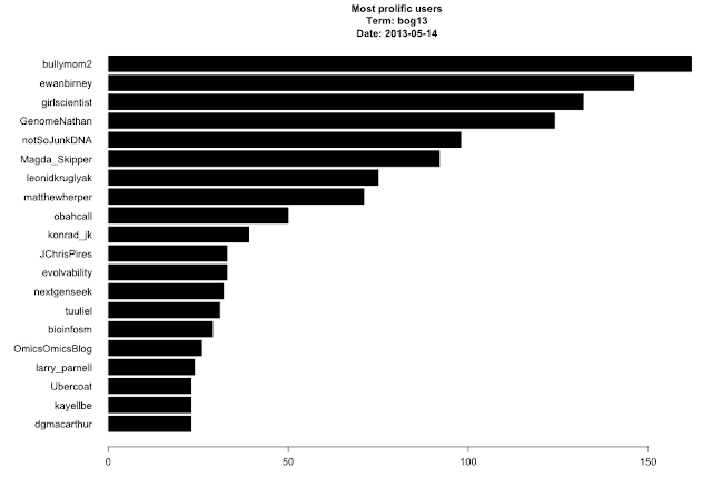
Here were the most prolific Tweeps - many of the usual suspects here, as well as a few new ones (new to me at least):

And finally, the requisite wordcloud:

More analysis

If you look in the analysis directory of the repo you'll find plots like these for other keywords (#rstats, metagenomics, rna-seq, and others to come). I would also like to do some sentiment analysis as Neil did in the ISMB post referenced above, but the sentiment package has since been removed from CRAN. I hear there are other packages for polarity analysis, but I haven't yet figured out how to use them. I've given you the code to do the mundane stuff (parsing the fixed-width files from t, for starters). I'd love to see someone take a stab at some further text mining / polarity / sentiment analysis!

twitterchive - archive and analyze results from a Twitter search

Three Metagenomics Papers for You

A handful of good metagenomics papers have come out over the last few months. Below I've linked to and copied my evaluation of each of these articles from F1000.

...

1. Willner, Dana, and Philip Hugenholtz. "From deep sequencing to viral tagging: Recent advances in viral metagenomics." BioEssays (2013). 

My evaluation: This review lays out some of the challenges and recent advances in viral metagenomic sequencing. There is a good discussion of library preparation and how that affects downstream sequencing. Alarmingly, they reference another paper that showed that different amplification methods resulted in detection of a completely different set of viruses (dsDNA viruses with LASL, ssDNA with MDA). The review also discusses many of the data management, analysis, and bioinformatics challenges associated with viral metagenomics.

...

2. Loman, Nicholas J., et al. "A Culture-Independent Sequence-Based Metagenomics Approach to the Investigation of an Outbreak of Shiga-Toxigenic Escherichia coli O104: H4Outbreak of Shiga-toxigenic Escherichia coli." JAMA 309.14 (2013): 1502-1510.

My evaluation: This paper is a groundbreaking exploration of the use of metagenomics to investigate and determine the causal organism of an infectious disease outbreak. The authors retrospectively collected fecal samples from symptomatic patients from the 2011 Escherichia coli O104:H4 outbreak in Germany and performed high-throughput shotgun sequencing, followed by a sophisticated analysis to determine the outbreak's causal organism. The analysis included comparing genetic markers from many symptomatic patients' metagenomes with those of healthy controls, followed by de novo assembly of the outbreak strain from the shotgun metagenomic data. This illustrates both the power, but the real limitations, of using metagenomic approaches for clinical diagnostics. Also see David Relman's synopsis of the study in the same JAMA issue

...

3. Shakya, Migun, et al. "Comparative metagenomic and rRNA microbial diversity characterization using archaeal and bacterial synthetic communities." Environmental microbiology (2013).

My evaluation: This study set out to compare shotgun metagenomic sequencing to 16S rRNA amplicon sequencing to determine the taxonomic and abundance profiles of mixed community metagenomic samples. Thus far, benchmarking metagenomic methodology has been difficult due to the lack of datasets where the underlying ground truth is known. In this study, the researchers constructed synthetic metagenomic communities consisting of 64 laboratory mixed genome DNAs of known sequence and polymerase chain reaction (PCR)-validated abundance. The researchers then compared metagenomic and 16S amplicon sequencing, using both 454 and Illumina technology, and found that metagenomic sequencing outperformed 16S sequencing in quantifying community composition. The synthetic metagenomes constructed here are publicly available (Gene Expression Omnibus [GEO] accession numbers are given in the manuscript), which represent a great asset to other researchers developing methods for amplicon-based or metagenomic approaches to sequence classification, diversity analysis, and abundance estimation.