Translational Bioinformatics Year In Review

Per tradition, Russ Altman gave his "Translational Bioinformatics: The Year in Review" presentation at the close of the AMIA Joint Summit on Translational Bioinformatics in San Francisco on March 26th.  This year, papers came from six key areas (and a final Odds and Ends category).  His full slide deck is available here.

I always enjoy this talk because it routinely points me to new collections of data and new software tools that are useful for a variety of analyses; as such, I thought I would highlight these resources from his talk this year.

GRASP: analysis of genotype-phenotype results from1390 genome-wide association studies and corresponding open access database
Some of you may have accessed the Johnson and O'Donnell catalog of GWAS results published in 2009.  This data set was a more extensive collection of GWAS findings than the popular NHGRI GWAS catalog, as it did not impose a genome-wide significance threshold for reported associations.  The GRASP database is a similar effort, reporting numerous attributes of each study.
A zip archive of the full data set (a flat file) is available here.


Effective diagnosis of genetic disease by computational phenotype analysis of the disease associated genome
This paper tackles the enormously complex task of diagnosing rare genetic diseases using a combination of genetic variants (from a VCF file), a list of phenotype characteristics (fed from the Human Phenotype Ontology), and a few other aspects of the disease.
The online tool called PhenIX is available here.


A network based method for analysis of lncRNA disease associations and prediction of lncRNAs implicated in diseases
Here, Yang et al. examine relationships between known long non-coding RNAs and disease using graph propagation.  Their underlying database, however, was generated using PubMed mining along with some manual curation.
Their lncRNA-Disease database is available here.


SNPsea: an algorithm to identify cell types, tissuesand pathways affected by risk loci
This tool is a type of SNP set enrichment, designed to specifically look at functional enrichment in the context of specific tissues and cell types.  The tool is a C++ executable, available for download here.
The data sources underlying the SNPsea algorithm are available here.


Human symptoms-disease network
Here Zhou et al. systematically extract symptom-to-disease network by exploting MeSH annotations.  They compiled a list of 322 symptoms and 4,442 diseases from the MeSH vocabulary, and document their occurrence within PubMed.  Using this disease-symptom network, the authors explore the biological underpinnings of certain symptoms by looking at shared genomic elements between diseases with similar symptoms.
The full list of ~130,000 edges in their disease-symptom network is available here.


A circadian gene expression atlas in mammals: implications for biology and medicine
This fascinating paper explores the temporal impact on gene expression traits from 12 mouse organs.  By systematically collecting transcriptome data from these tissues at two hour intervals, the authors construct a temporal atlas of gene expression, and show that 43% of proteins have a circadian expression profile.
The accompanying CircaDB database is available online here.


dRiskKB: a large-scale disease-disease riskrelationship knowledge base constructed frombiomedical text
The authors of dRiskKB use text mining across MEDLINE citations using a controlled disease vocabulary, in this case the Human Disease Ontology, to generate pairs of diseases that co-occur with specific patterns in abstract text. These pairs are ranked with a scoring algorithm and provide a new resource for disease co-morbidity relationships.
The flat file data driving dRiskKB can be found online here.


A tissue-based map of the human proteome
In this major effort, a group of investigators have published the most detailed atlas of human protein expression to date.  The transcriptome has been extensively studied across human tissues, but it remains unclear to what extent transcriptional activity reflects translation into protein.  But most importantly, the data are searchable via a beautiful website.
The underlying data from the Human Protein Atlas is available here.

Do your "data janitor work" like a boss with dplyr

Data “janitor-work”

The New York Times recently ran a piece on wrangling and cleaning data:

“For Big-Data Scientists, ‘Janitor Work’ Is Key Hurdle to Insights”

Whether you call it “janitor-work,” wrangling/munging, cleaning/cleansing/scrubbing, tidying, or something else, the article above is worth a read (even though it implicitly denigrates the important work that your housekeeping staff does). It’s one of the few “Big Data” pieces that truly appreciates what we spend so much time doing every day as data scientists/janitors/sherpas/cowboys/etc. The article was chock-full of quotable tidbits on the nature of data munging as part of the analytical workflow:

It’s an absolute myth that you can send an algorithm over raw data and have insights pop up…

Data scientists … spend 50-80% of their time mired in this more mundane labor of collecting and preparing unruly digital data, before it can be explored for useful nuggets.

But if the value comes from combining different data sets, so does the headache… Before a software algorithm can go looking for answers, the data must be cleaned up and converted into a unified form that the algorithm can understand.

But practically, because of the diversity of data, you spend a lot of your time being a data janitor, before you can get to the cool, sexy things that got you into the field in the first place.

As data analysis experts we justify our existence by (accurately) evangelizing that the bottleneck in the discovery process is usually not data generation, it’s data analysis. I clarify that point further with my collaborators: data analysis is usually the easy part — if I give you properly formatted, tidy, and rigorously quality-controlled data, hitting the analysis “button” is usually much easier than the work that went into cleaning, QC’ing, and preparing the data in the first place.

To that effect, I’d like to introduce you to a tool that recently made its way into my data analysis toolbox.

dplyr

Unless you’ve had your head buried in the sand of the data analysis desert for the last few years, you’ve definitely encountered a number of tools in the “Hadleyverse.” These are R packages created by Hadley Wickham and friends that make things like data visualization (ggplot2), data management and split-apply-combine analysis (plyr, reshape2), and R package creation and documentation (devtools, roxygen2) much easier.

The dplyr package introduces a few simple functions, and integrates functionality from the magrittr package that will fundamentally change the way you write R code.

I’m not going to give you a full tutorial on dplyr because the vignette should take you 15 minutes to go through, and will do a much better job of introducing this “grammar of data manipulation” than I could do here. But I’ll try to hit a few higlights.

dplyr verbs

First, dplyr works on data frames, and introduces a few “verbs” that allow you to do some basic manipulation:

• filter() filters rows from the data frame by some criterion
• arrange() arranges rows ascending or descending based on the value(s) of one or more columns
• select() allows you to select one or more columns
• mutate() allows you to add new columns to a data frame that are transformations of other columns
• group_by() and summarize() are usually used together, and allow you to compute values grouped by some other variable, e.g., the mean, SD, and count of all the values of $y separately for each level of factor variable $group.

Individually, none of these add much to your R arsenal that wasn’t already baked into the language in some form or another. But the real power comes from chaining these commands together, with the %>% operator.

The %>% operator: “then”

This dataset and example was taken directly from, and is described more verbosely in the vignette. The hflights dataset has information about more than 200,000 flights that departed Houston in 2011. Let’s say we want to do the following:

1. Use the hflights dataset
2. group_by the Year, Month, and Day
3. select out only the Day, the arrival delay, and the departure delay variables
4. Use summarize to calculate the mean of the arrival and departure delays
5. filter the resulting dataset where the arrival delay or the departure delay is more than 30 minutes.

Here’s an example of how you might have done this previously:

filter(
  summarise(
    select(
      group_by(hflights, Year, Month, DayofMonth),
      Year:DayofMonth, ArrDelay, DepDelay
    ),
    arr = mean(ArrDelay, na.rm = TRUE),
    dep = mean(DepDelay, na.rm = TRUE)
  ),
  arr > 30 | dep > 30
)

Notice that the order that we write the code in this example is inside out - we describe our problem as: use hflights, then group_by, then select, then summarize, then filter, but traditionally in R we write the code inside-out by nesting functions 4-deep:

filter(summarize(select(group_by(hflights, ...), ...), ...), ...)

To fix this, dplyr provides the %>% operator (pronounced “then”). x %>% f(y) turns into f(x, y) so you can use it to rewrite multiple operations so you can read from left-to-right, top-to-bottom:

hflights %>%
  group_by(Year, Month, DayofMonth) %>%
  select(Year:DayofMonth, ArrDelay, DepDelay) %>%
  summarise(
    arr = mean(ArrDelay, na.rm = TRUE),
    dep = mean(DepDelay, na.rm = TRUE)
  ) %>%
  filter(arr > 30 | dep > 30)

Writing the code this way actually follows the order we think about the problem (use hflights, then group_by, then select, then summarize, then filter it).

You aren’t limited to using %>% to only dplyr functions. You can use it with anything. E.g., instead of head(iris, 10), we could write iris %>% head(10) to get the first ten lines of the built-in iris dataset. Furthermore, since the input to ggplot is always a data.frame, we can munge around a dataset then pipe the whole thing into a plotting function. Here’s a simple example where we take the iris dataset, then group it by Species, then summarize it by calculating the mean of the Sepal.Length, then use ggplot2 to make a simple bar plot.

library(dplyr)
library(ggplot2)
iris %>%
  group_by(Species) %>%
  summarize(meanSepLength=mean(Sepal.Length)) %>%
  ggplot(aes(Species, meanSepLength)) + geom_bar(stat="identity")

Once you start using %>% you’ll wonder to yourself why this isn’t a core part of the R language itself rather than add-on functionality provided by a package. It will fundamentally change the way you write R code, making it feel more natural and making your code more readable. There's a lot more dplyr can do with databases that I didn't even mention, and if you're interested, you should see the other vignettes on the CRAN package page.

As a side note, I’ve linked to it several times here, but you should really check out Hadley’s Tidy Data paper and the tidyr package, vignette, and blog post.

dplyr package: http://cran.r-project.org/web/packages/dplyr/index.html

dplyr vignette: http://cran.rstudio.com/web/packages/dplyr/vignettes/introduction.html

dplyr on SO: http://stackoverflow.com/questions/tagged/dplyr

​

There is no Such Thing as Biomedical "Big Data"

At the moment, the world is obsessed with “Big Data” yet it sometimes seems that people who use this phrase don’t have a good grasp of its meaning.  Like most good buzz-words, “Big Data” sparks the idea of something grand and complicated, while sounding ordinary enough that listeners feel like they have an intuitive understanding of the concept.  However "Big Data" actually carries a specific technical meaning which is getting lost as the term becomes more popular.    

The phrase's predecessor, "Data Mining" was equally misunderstood.  Originally called "database mining" (a subsequently trademarked term), the term "Data Mining" became common during the 1990s as many businesses rapidly adopted the use of relational database management systems (RDMS) such as Oracle.  RDMS store, optimize, and manage large amounts of data on physical disks for the purpose of rapid search, retrieval and update.  These large collections of data enabled businesses to extract new knowledge useful to their business practices by examining patterns within their data.  Data mining refers to a collection of algorithms that attempt to extract knowledge (in the form of rules or associations) from large amounts of data by processing it in place on the disk, either within the RDMS or within large flat files.  This is an important distinction, as the optimization and speed of algorithms that access data from the disk can be quite different from those which examine data within active memory.

A great example of data mining in practice is the use of frequent itemset mining to target customers with coupons and other discounts.  Ever wonder why you get a yogurt coupon at the register when you check out?  That’s because across thousands of other customers, a subgroup of people with shopping habits similar to yours consistently buys yogurt, and perhaps with a little prompting the grocery vendor can get you to consistently buy yogurt too.

As random access memory (RAM) prices dropped (and virtual memory procedures within operating systems improved), it became much more feasible to process even extremely large datasets within active memory, reducing the need for algorithmic refinements necessary for disk-based processing. But by then, "data mining" (marketed as a way to increase business profits) had become such a popular buzz-word, it was used to refer to any type of data analysis. 

 

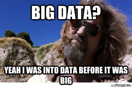
In fact, it has been tacked on to numerous books and publications about machine learning methods purely for marketing purposes.  Supposedly even some publishers have modified the titles of machine learning books to include the phrase “data mining” with the hope that it will improve sales.  As a result, the colloquial meaning of data mining has become "a vaguely defined way to discover patterns in data".  To me, this is a tragedy because we have lost a degree of specificity in our language simply because “data mining” sounds cool and profitable.   

Zoom forward to the present day and we see history repeating with the phrase “big data”.  With the increasing popularity of cell phone technologies and the internet, the last decade has seen a dramatic growth in data generated by commercial transactions and online websites.   Many of these large companies (think Google's Search Indices or Facebook and LinkedIn network data) generate data on such a large scale that it cannot be managed within traditional database systems.  These groups have instead turned to large computing clusters that distribute the data over many, many separate machines and file systems.  Partitioning data in this way requires a new class of algorithms that can take advantage of the fact that individual processing units (or nodes of a computing cluster) house their own subset of the overall data.  This is a fundamental paradigm of “Big Data” algorithms, making it distinct from other machine learning and data mining techniques.

A great example of a “Big Data” programming model is the MapReduce framework developed by Google.  The basic idea is that any data manipulation step has a Map function that can be distributed over many, many nodes on a computing cluster that then filter and sort their own portion of the data.  A Reduce function is then performed that combines the selected and sorted data entries into a summary value.  This model is implemented by the popular Big Data system Apache Hadoop.

All of the fuss over “Big Data” is driven by these massive producers of data (on the order of hundreds of terabytes a day), yet the ideas behind “Big Data” are being applied on much smaller datasets even when they are not necessary.  In fact, a rather amusing read from Microsoft Research describes the overhype of “Big Data” algorithms and the surprisingly few analytic operations that truly need these approaches.  The hype is alive and well in the medical and biological research community as well.  In fact, there is an NIH initiative to fund “Big Data to Knowledge”.  I'm the first to cheer for projects dedicated to large-scale data analysis, but by nearly any definition, right now there is no such thing as biomedical Big Data.     

There are certainly processes in biomedical research that produce large amounts of data – first among them is next generation sequencing technology.  In sequencing studies, the raw data from sequencers is aligned and processed to extract the meaningful information (i.e. SNP and CNV calls).  After processing, a full human genome will nearly fit on a floppy disk, which hardly qualifies as "Big Data".  While there may be some interest in storing the raw underlying data (sequence reads), it may prove much more cost effective to simply regenerate the data.  Based on an excellent analysis by Glenn Lockwood, storing four weeks worth of HiSeq X10 raw data may cost nearly $10,000 a month.  If instead we store derived features from the raw data, data storage and manipulation is on the order of typical imputed GWAS.  There will undoubtedly be a desire to reprocess this raw sequence data with new algorithms, but unless storage prices drop rapidly, regenerating the data will be more cost-effective than storage.  Therefore, in my opinion right now the closest thing to qualifying as Big Data would be large multi-center electronic medical record systems, yet even these are typically managed by large-scale relational database systems.

So in practice, our grants will be filled with mentions of Big Data, Web 3.0, "thinking outside the box", value added, hype/innovation, but in reality biomedical sciences are nowhere near approaching the scale needed for real Big Data approaches.    

Thanks to Alex Fish for her thoughtful edits.